ZJUNlict Extended Team Description Paper for RoboCup 2019
Zheyuan Huang, Lingyun Chen, Jiacheng Li, Yunkai Wang, Zexi Chen, Licheng Wen, Jianyang Gu, Peng Hu, Rong Xiong
Zhejiang University, Zheda Road No.38, Hangzhou, Zhejiang Province, P.R.China
Abstract For the Small Size League of RoboCup 2018, Team ZJUNLict has won the champion and therefore, this paper thoroughly described the devotion which ZJUNLict has devoted and the effort that ZJUNLict has contributed. There are three mean optimizations for the mechanical part which accounted for most of our incredible goals, they are "Touching Point Optimization", "Damping System Optimization", and "Dribbler Optimization". For the electrical part, we realized "Direct Torque Control", "Efficient Radio Communication Protocol" which will be credited for stabilizing the dribbler and a more secure communication between robots and the computer. Our software group contributed as much as our hardware group with the effort of "Vision Lost Compensation" to predict the movement by kalman filter and a new interception prediction algorithm to achieve some skills.
1 Introduction
This paper is organized as follows: First of all, the major optimization of our mechanical architecture which accounted for most of our incredible goals are described in section 2. They are "Touching Point Optimization", "Damping System Optimization", and "Dribbler Optimization". The detailed tasks for the electrical system include driving motors, wireless communication, charging and discharging capacitors for shooting and chipping, which are described in section 3. Our detailed improvements in vision module are described in section 4, which enables us to play the game under a terrible vision situation. Some skills based on the new interception prediction algorithm are explained in section 5.
2 ZJUNlict New Dribbler Design
2.1 Typical Dribblers and Existing Problems
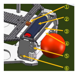
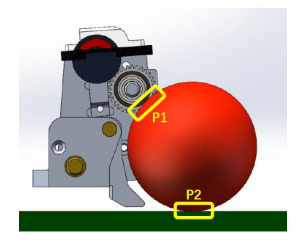
The small size league robots do not really have foot like human beings. Instead, they have dribblers. A dribbler is a device that can help dribble and catch the ball. As shown in Fig. 1, a typical dribbler has the following features. A shelf connects 2 side plates and the dribbling motor is fixed on one side plate. Between the 2 side plates is a cylindrical dribbling-bar driven by the dribbling motor. The whole device has only one degree of freedom of rotation and the joints are fixed on the robot flame. Usually there is a unidirectional springdamping system locates between the shelf and the robot frame to help improve the stability of dribbling as well as absorbing the energy when catching the ball. The dribbling-bar driven by the dribbling motor provides torque to make the ball spin backward when the contact between the ball and dribbling-bar exits so that the ball can be 'locked' by this device in ideal conditions. And the carpet provides supporting force and frictional force and therefore there are 2 touch points on the ball and in this paper we called it a 2-touch-point model (Fig. 2). For the motor control, most teams try to keep the dribbling-bar at a constant rotational speed when dribbling the ball and therefore it is actually an open loop control mode for dribbling. Unfortunately, this 2-touch-point dribbler with unidirectional spring-damping system and passive control mode does not provide ideal dribbling performances. It is quite easy for the ball to bounce back and forth when launching the dribbling motor. The device might also not absorb enough kinetic energy of the moving ball when catching it so it will bounce back and there occurs a catching failure. Actually it is also hard to greatly improve its performance by simply changing the material of dribbling-bar, adjusting the damping and stiffness of the spring-damping system or adjusting the rotational speed of motor. This structure has natural defects with passive control mode.
![Fig. 3. Energy Absorbing by Creating a Dual Freedom [7]](/tdps/soccer_smallsize__2019__ZJUNlict/_page_2_Picture_3.jpeg)
2.2 Dribbler Improvements
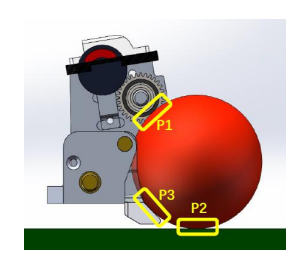
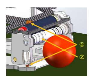
Considering the purpose above, we devoted ourselves on the dribbler. Firstly, we adjust the geometry parameters of the device so that the ball can touch the chip shovel in steady state, which means both carpet and chip shovel can provide supporting force and frictional force to the ball so we called it a 3-touch-point model (Fig. 4). Normally the dynamic friction coefficient between the ball-carpet surface is greater than that of the ball-chip shove surface. Therefore, when the ball driven by the dribbling-bar moves from the carpet on to the chip shove surface, there will be a sudden drop of frictional force, and the ball will be pushed back on the carpet. And once the ball touches the carpet, there will be a sudden increase of frictional force, the ball will be driven onto the chip shove again. In this kind of state, the amount of spring compression will not change much so that the dribbling system will enter a periodical dynamic steady state. In contrast, with a 2-touch-point system, the friction force will not change much so the ball will enter much more into the dribbler and there will be a bigger compression of the spring-damping system. Therefore the ball will also be pushed back more and totally the bouncing amplitude will be much greater, or even the ball will bounce off the dribbler. In addition, we found that there will be a hard contact between the side plates and the baseplate when the dribbler hits the baseplate. So besides the foam between the shelf and the robot frame, we stick 1.5 mm thick tape between the side plates and baseplate so there will be a soft contact when the dribbler hits the baseplate. Actually this design makes up a bidirectional spring-damping system (Fig. 5) and improves the dynamic behavior of the dribbler. Hopefully it can reduce the bouncing amplitude of the ball when dribbling as well as absorbing more kinetic energy when catching the ball. To improve the dribbling performance when the robot rotates or moves laterally, we also made a dribbling-bar with screw using 3D printing rubber so that it can provide lateral force to the ball when dribbling as shown in Fig.5. Another key point to make this device better is to change the passive rotational speed control mode to active torque control mode. Instead of keeping the rotational speed with a constant value, we control the motor torque constant according to the current feedback. With the innovations above, we create a quite good active control dribbler.
2.3 Tests and Verifications
According to the catching ability tests, the typical 2-touch-point dribbler with unidirectional spring-damping system could catch a ball with coming speed up to 3m/s and the new 3-touch-point dribbler with bidirectional spring-damping system could catch a ball with coming speed up to 8.5m/s. The results were quite clear that the new dribbler has better dribbling and catching ability. In addition, we made simple tests to see the effect of screw added on the dribbling bar. The dribbling motor was launched and after the dribbling entering the steady state, we made the robot spin around. The rotational acceleration is 20deg/s² and the rotation speed was recorded at the time the ball left the dribbler. This simple test was carried out 10 times for both smooth dribbling-bar and screw dribblingbar, which were made by some same material. As show in Tabel.1, the average escape speed of smooth dribbling-bar is 402deg/s and for the screw dribblingbar is 622deg/s. So it was proved that the design of screw could improve the dynamic dribbling performance of dribbler.
Table 1. Dynamic Dribbling Ability Comparison Between Smooth Dribbling-bar and Screw Dribbling-bar
| Dribbling-bar Type | 1 | 2 | 3 | 4 | 5 | 6 | 7 | 8 | 9 | 10 | Average |
|---|---|---|---|---|---|---|---|---|---|---|---|
| Smooth Dribbling-bar (deg/s) | 400 | 340 | 380 | 360 | 380 | 420 | 400 | 420 | 400 | 520 | 402 |
| Screw Dribbling-bar (deg/s) | 600 | 580 | 580 | 580 | 620 | 680 | 620 | 680 | 640 | 640 | 622 |
3 Electrical System
3.1 Overview
For a typical Small Size League robot, the electrical system is responsible for the overall control of the hardware based on commands sent by a team's strategy program. The detailed tasks for the electrical system include driving motors, wireless communication, charging and discharging capacitors for shooting and chipping. There are three configurations of electrical systems shown in the Table 2 below currently used in ZJUNlict robots. The single Cyclone III FPGA configuration was adopted since 2012 and explained in 2013 and 2014 champion papers [1, 2]. The FPGA handles both motor control and other tasks such as communication and motion sensor fusion based on embedded Nios II processor. The micro-controller STM32F407 was added to take over tasks other than motor control since late 2017 [4]. Since 2018, a single micro-controller STM32H743 capable of operation frequency up to 400MHz combined with five BLDC controller Allegro A3930 was able to handle all the tasks. Other improvements include increasing each encoder's counts per revolution (CPR) to increase motor lowspeed control performance, implementation of the accelerometer and compass to achieve more accurate motion tracking and switching to nRF24L01+ wireless IC to deliver higher bandwidth communication with better signal sensitivity.
Table 2. ZJUNlict Electrical System Configurations
| Configuration | Since 2012 | Since 2017 | Since 2018 |
|---|---|---|---|
| Microcontroller | Cyclone III EP3C25 | Cyclone III EP3C25 STM32F407 | STM32H743 |
| Driving Motors | Maxon EC-45 50W | ||
| Dribbling Motor | Maxon EC-16 30W | ||
| Encoder | US Digital E4T, 500 CPR | 1000 CPR | |
| BLDC Driver | IR2103S | Allegro A3930 | |
| Motion Sensors | Gyroscope | Gyroscope, Accelerometer, Compass | |
| MOSFETs | IRFR1205 | IRF8313 | |
| Wireless IC | nRF2401A | 2 x nRF24L01+ | |
| Kick Charge IC | UC3843 |
3.2 Torque Control for Dribbler Motor
The torque control model for dribbler motor is based on team Skuba's design [8–10]. The motor's dynamic equation is derived from Maxon motor data [5].
$$\tau_m = \left(\frac{k_m}{R}\right) \cdot u - \left(\frac{k_m}{R \cdot k_n}\right) \cdot \omega$$
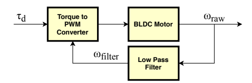
where, τᵐ is the output torque of the motor, kᵐ is the torque constant of the motor, R is the resistance of the motor, u is the input voltage, kⁿ is the motor speed constant, ω is the angular velocity of the motor. Equation 1 shows the relationship between output torque τm, input voltage u and angular velocity ω. The diagram for the torque controller is shown in the Fig. 6 below. The angular velocity ωraw is acquired through the hall sensor. A low pass filter is used to reduce the noise in the velocity measurement. The desired torque τᵈ is set through the simulation result of the ADAMS model.
3.3 Efficient Radio Communication Protocol
The communication quality becomes a pressing problem when the competition requires a larger field and more robots. For a typical nRF24L01+ wireless package (maximum 32 bytes) consists of 5 bytes receiver address, 2 bytes CRC and 25 bytes user payload. Compared with other teams' communication protocol [6, 7] which often requires one package for each robot, the presented efficient communication protocol is shown in the Table 3 significantly reduces the package amount required in each control period. Apart from 1 byte package header indicates the package type and robot existence in each package, each robot takes up to 6 bytes for the velocity, dribbler and kick command. For 25 bytes user payload, each package is able to control up to 4 robots. The bandwidth of nRF24L01+ can also be set to 1Mbits/s and 250kbits/s which requires fewer frequency bandwidth. By reducing the communication traffic in each control period and frequency bandwidth both reduces the possibility of radio interference.
Table 3. ZJUNlict Radio Communication Protocol
| Byte | bit | 7 | 6 | 5 | 4 | 3 | 2 | 1 | 0 |
|---|---|---|---|---|---|---|---|---|---|
| Head | 0 | Package Type | Robot 1 Exist? | Robot 2 Exist? | Robot 3 Exist? | Robot 4 Exist? | |||
| Robot 1 Config | 1 | Report? | Dribble Strength Shoot:0 Chip:1 (0-3) | Number of Robot 1 | |||||
| 2 | 0:+ 1:- | Speed Vx Unit: 1 cm/s | |||||||
| 3 | 0:+ 1:- | Speed Vy Unit: 1 cm/s | |||||||
| 4 | 0:+ 1:- | Rotation Speed ω Unit: 1/40 rad/s | |||||||
| 5 | Speed Vx and Vy High 2bits | Rotation Speed High 4 bits | |||||||
| 6 | Kick Power (7 bits) |
4 SSL Vision Solution
4.1 Existing Problems
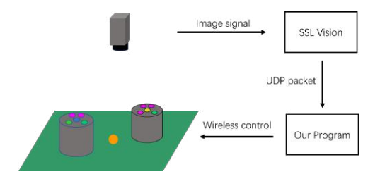
The existing image recognition system of SSL is shot by cameras (780 × 580 YUV422 60Hz) which suspended about 4m above the field. After image acquisition, the vision software provided by SSL official performs color block recognition progress on the ball (orange) and the color code on the top of each robot. The software determines the robot's information (team, id, position and orientation) based on the color code combination at the top of robot, and recognizes the position of the ball based on the orange color patch. Finally the robot and ball information is transmitted to our program for processing in the form of UDP packets.
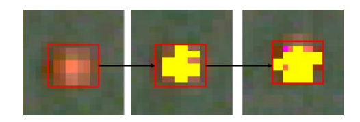
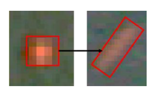
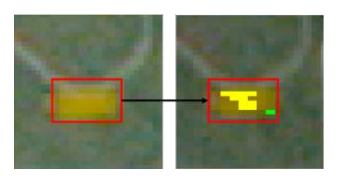
As the picture (Fig. 7) shows the basic process of the whole SSL vision system. This image system has been used in the SSL competition for around ten years. As the size of the field continues to enlarge, the number of cameras on the field has also increased from 2 to 8(in this year's competition). Using color block recognition algorithm accordingly will cause the image processed by the graphic processor to survive the following problems:
4.2 Solution Introduction
Our image solution provides a code framework that covers the various special cases described above, allowing us to perform algorithmic processing for each situation. After receiving the UDP packet sent by the Graphic Processor, the program will automatically judge the current image quality and suspicious conditions for subsequent algorithm processing.
Noise Cancellation For raw data containing noise, we use a Kalman filter considering noise cancellation.
In order to use the Kalman filter to estimate the internal state of a process given only a sequence of noisy observations, one must model the process in accordance with the framework of the Kalman filter. This means specifying the following matrices:
- Fk, the state-transition model;
- and sometimes Bk, the control-input model, for each time-step, k, as described below.
The Kalman filter model assumes the true state at time k is evolved from the state at (k − 1) according to
$$x_k = F_k x_{k-1} + B_k u_k + w_k$$
where Fᵏ is the state transition model which is applied to the previous state xk−1; Bᵏ is the control-input model which is applied to the control vector uk; wᵏ is the process noise which is assumed to be drawn from a zero mean multivariate normal distribution, N , with covariance, Qᵏ : wᵏ ∼ N (0, Qk)
At the same time, because the data noise is effectively eliminated after Kalman filtering, we can also rely on these data for velocity estimation and position prediction.
Object Confidence In order to solve the misjudgment and missed information of the original image itself, we maintained the confidence of the ball and the robot on the field.
$$P_{o,t} = P_{o,t-1} + P(seen, t) - P(lost, t), 0 \le P_o \le 1$$
The above is the mathematical expression of confidence, where:
- Po,t is the confidence of the object o at time t. We set 0 as the initial value of Po,t
- P(seen, t) is the probability rise constant of the object o appearing in the image at time t
- P(lost, t) is the probability reduction coefficient of the object disappearing on the image at time t
According to the above formula, we set a confidence threshold of Pv, then
$$object = \begin{cases} valid, & P_{o,t} > P_v \ invalid, & P_{o,t} \le P_v \end{cases}$$
This solution effectively eliminates the effects of loss of objects due to cameras, light, and the like. At the same time, interference caused by similar objects such as skin is not considered a valid object because its duration is short and its confidence is lower than the confidence threshold.
Camera Parameter Identification Due to the complexity of multiple camera coverage areas on the site, we have adopted an algorithm that automatically identifies camera parameters. While continuously receiving image information, we continuously calculate and update the coverage area, parameters, etc. of the camera.
When an object appears in the field of view of multiple cameras at the same time, we will calculate its actual position by the following formula: ¯rreal
$$\bar{r}{real} = \frac{\sum{i=1}^{k} \frac{\bar{r}{i} - \bar{r}{cam_{i}}}{R_{cam_{i}}} r_{i}}{\sum_{i=1}^{k} \frac{\bar{r}{i} - \bar{r}{cam_{i}}}{R_{cam_{i}}}}$$
Among them
- r¯camⁱ is the projection coordinate of camera i
- Rcamⁱ is the coverage distance of camera i
- k is the number of cameras that can see the current object
4.3 Results
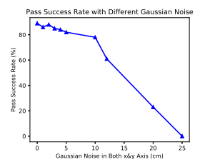
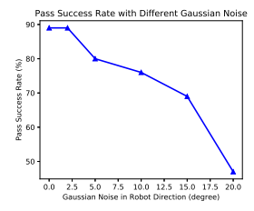
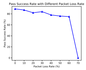
We use the simulation software grSim to test the actual effect of our image module. GrSim can adjust the noise (Gaussian noise) and packet loss rate of the original output image to simulate the effect of real games.
We use the pass success rate to reflect the accuracy of our image module handlers, and we will test the success rate of 100 passes in the current environment.
5 Interception Prediction Algorithm and Application
5.1 Robot Arrival Time Prediction
In our system, we adopted the method used in [11]. First, we carried out RRT global planner, and then the velocity planner based on the path points generated by RRT. For the velocity planner, we use trapezoidal programming. Since it is the omnidirectional wheel that we used, we decompose the translational speed and rotational speed into a 2d planner and a 1d planner. Then, we decompose the translational velocity into two directions with the orientation from the starting location to the target location as the X-axis, which is beneficial for the robot to achieve the maximum velocity in the x-direction, while the velocity in the y-direction decreases to zero as soon as possible. This will reduce the coupling between the two directions. Therefore, we're basically doing three 1d planner, and then combine them together. For each 1d planner, we will use the maximum acceleration and maximum deceleration under ideal conditions to make a trapezoidal program. Therefore, it could reach the target location with the optimal time, which we can accurately predict.
5.2 Search-Based Interception Prediction Algorithm
On the basis of realizing the algorithm of accurately predicting the robot's arrival time to a certain destination, we developed a search-based algorithm that predicts the shortest interception time and the best interception point for the robots. In one actual game, according to the movement ability of both sides, we will make an interception prediction for each robot on both sides of the field in each frame. This is very important for the realization of our single robot skills and the realization of multi-robot attack and defense conversion. In order to ensure the feasibility and real-time of this process, we use the search-based strategy to search the time at equal intervals with a fixed minimum interval of ∆t(such as 1/60 of a second). At a certain moment t, we obtain the location and speed of both the robot and the ball, then calculate the locationPⁱ that the ball can reach at any time t + i∆t(i = 0, 1, 2, 3, ...) in the future under the action of the frictional force of the field in a straight line motion with uniform deceleration(the acceleration of the ball can be obtained according to the measured friction coefficient of the field). Then, starting from i = 0, it traversed the search points to predict the time Tⁱ that would take a robot to reach the pointPⁱ . If Tᵏ ≤ t + k∆t is satisfied after the k-th interval, point Pᵏ is considered to be the best interception point Pbest of the robot, and Tᵏ is the shortest interception time Tbest of the robot. Algorithm 1 shows the specific algorithm pseudocode.
There are two extreme cases. One is that the ball has already stopped before the robot intercepts the ball. At this time, the location where the ball stops is the optimal interception location, and the time when the robot reaches the location is the shortest interception time. Another is that the ball has been out of bounds before the robot intercepted it. At this time, in order to ensure that the algorithm can always get a solution, we take the out of bounds location as the best interception location, and the time to the out of bounds location as the shortest interception time. If the prediction of interception time is relatively conservative, such as adding fixed adjustment time Tᵐ to the predicted robot arrival time Tⁱ , to ensure a higher success rate of the robot to intercept the ball. It will be found in the actual application that the robot will run more directly to the boundary to intercept the ball.
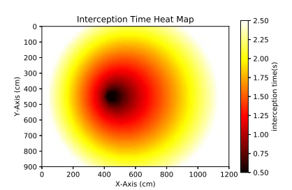
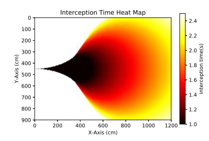
Fig. 14 and Fig. 15 shows the interception time of a stationary robot at different positions under two different ball speeds. Darker areas represent shorter interception time, while lighter areas represent longer interception time. In Fig. 14, the initial position of the ball is (400cm, 450cm), and ball speed is low (1m/s), so at a certain time, the closer the robot gets to the ball, the less time it has to intercept the ball. However, when ball speed is high, it has different conclusion. In Fig. 15, the initial position of the ball is (0cm, 450cm), and ball speed is high (4m/s). Robot cannot intercept the ball in most places on the left side, and there is an obvious boundary. If the position of the robot is within the boundary(i.e. the dark area), it can intercept the ball in a short time, but if not, it will cost much, and may never intercept the ball before it out of the field. In the old saying of China, it is called "A little error may lead to a large discrepancy".
Algorithm 1 Search-Based Interception Prediction:
Require: ∆t, ball initial position P0 and velocity v0, robot initial position Pr and velocity vr
  k ← 0
  repeat
    Pk ← predictBallPosition(P0, v0, k∆t)
    Tk ← predictRobotArrivalTime(Pr, vr, Pk)
    k ← k + 1
  until Tk ≤ k∆t or Pk out of the field
  Pbest ← Pk
  Tbest ← Tk
In [3] we developed a "FSM-based Role Matching" mechanism, using the square of the distance between the current positions of the robots and expected roles' target positions as the cost function. Considering the above situation, it is actually wrong when math robots to intercept the ball if we choose the ball position as the target position. A better way is using the time that robots move from the current positions to the target as a loss function, and if the target is a ball, using Algorithm 1 can match an optimal robot to get the ball, that will improve our ball possession rate.
5.3 Implementation of Intercept Ball Skill
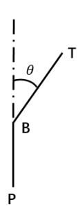
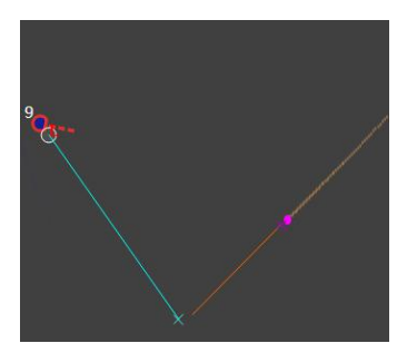
Since we can predict robot optimal interception position, we developed a dynamic interception skill based on our robot location, optimal interception location, and kicking location. As shown in the Fig. 16, assuming that the location of our robot is location P, the predicted optimal interception location is location B, the kicking location is location T, and the Angle between PB and BT is $\theta$ , we choose different interception methods according to the absolute value of $\theta$ . If the absolute value of $\theta$ is less than 45 degrees, we select the "Chase Ball" skill, which is chasing the ball forward and kicking to the target location; If it is between 45 and 120 degrees, we select the "Intercept Ball" skill. We intercept the ball, then turn around and shoot at the target location. If it is greater than 120 degrees, we select the "Touch Ball" skill, run to the ball and kick the ball directly to the target location.
5.4 Implementation of Marking Skill
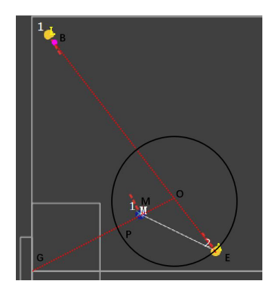
Based on the implementation of the interception prediction algorithm, we have developed a new "Marking" skill based on the best interception location and the shortest interception time of both sides.
Fig. 18 shows an application of this skill. Let us assume that we are on the blue side, the yellow robot No.1 is now controlling the ball, location B is the location of the ball, the yellow robot No.2 is the possible ball catching robot, location E is its location, and G is the center location of the goal. Since the robot generally moves at a low speed when passing and catching the ball, we can assume that the robot on the field is stationary. We assume that the ball will move along ray BE at the maximum speed from location B at the next moment, and the yellow robot No.2 will intercept the ball according to the maximum movement ability of the enemy. According to the interception prediction algorithm, the optimal interception location of the yellow robot No.2 can be calculated at location O. Draw a circle O with location O as the center of the circle and the length of segment OE as the radius. Assuming that our robot has the same movement ability as the enemy robot, as long as our robot No.1 is in circle O, it can intercept the ball before the yellow robot No.2. In order to balance the grab and defense, we line segment OG, and segment OG intersects the circle O at location P. We will choose the position like M of our No.1 robot station on the segment OP near the location P.
The application of this skill allows us more likely to grab the ball passing of the other side, thus greatly improving our ball possession rate.
6 Conclusion
In this paper, we have introduced four main optimizations in both hardware section and software section in the competition last year. Our future task is to increase the intelligence and scalability of our system. We are working on changing our microcontroller from FPGA to STM32. Deep reinforcement learning(DRL) and CUDA will also be used in our algorithm to improve the performance of our robots. In the robot control part, we are trying to use B´ezier curve and TEB[12] to improve our motion module, reduce collisions and make the trajectory smoother.
References
- Zhao, Yue, et al.: ZJUNlict: RoboCup 2013 small size league champion. Robot Soccer World Cup. Springer, Berlin, Heidelberg, 2013.
- Li, Chuan, et al.: Zjunlict: Robocup 2014 small size league champion. Robot Soccer World Cup. Springer, Cham, 2014.
- Zhao, Yue, et al.: ZJUNlict Team Description Paper for RoboCup 2014. RoboCup Wiki as team description of ZJUNlict, João Pessoa, Brazil, accessed Feb 5 (2014): 2019.
- Lingyun Chen, et al.: ZJUNlict Extended Team Description Paper for RoboCup 2018. RoboCup Wiki as extended team description of ZJUNlict, Montreal, Canada, accessed March 6 (2018): 2019.
- Kafader Urs.: Motor data and operating ranges of maxon DC motors. Maxon Motor AG, Sachseln, Switzerland (2010)
- Andre Ryll, Mark Geiger, Nicolai Ommer, Arne Sachtler, Lukas Magel.: TIGERs Mannheim Extended Team Description for RoboCup 2016. RoboCup Wiki as extended team description of TIGERs Mannheim team, Leipzig, Germany, accessed April 18 (2016): 2019.
- Andre Ryll, Mark Geiger, Chris Carstensen, Nicolai Ommer.: TIGERs Mannheim Extended Team Description for RoboCup 2018. RoboCup Wiki as extended team description of TIGERs Mannheim team, Montreal, Canada, accessed March 6 (2018): 2019.
- Sukvichai, Kanjanapan, Piyamate Wasuntapichaikul, and Yodyium Tipsuwan.: Implementation of torque controller for brushless motors on the omni-directional wheeled mobile robot. ITC-CSCC. 2010.
- Chaiso, Krit, and Kanjanapan Sukvichai.: Skuba 2011 Extended Team Description. RoboCup Wiki as extended team description of SKUBA team, Istanbul, Turkey, accessed Feb 21 (2011): 2019.
- Sukvichai, Kanjanapan, Teeratath Ariyachartphadungkit, and Krit Chaiso.: Robot hardware, software, and technologies behind the SKUBA robot team. Robot Soccer World Cup. Springer, Berlin, Heidelberg, 2011.
- Bruce, James R. Real-time motion planning and safe navigation in dynamic multirobot environments. No. CMU-CS-06-181. CARNEGIE-MELLON UNIV PITTS-BURGH PA SCHOOL OF COMPUTER SCIENCE, 2006.
- Rösmann, Christoph, et al. "Trajectory modification considering dynamic constraints of autonomous robots." ROBOTIK 2012; 7th German Conference on Robotics. VDE, 2012.