ER-Force 2020 Extended Team Description Paper

Andreas Wendler, Tobias Heineken

Friedrich-Alexander-Universität Erlangen-Nürnberg (FAU), Faculty of Engineering, Department of Computer Science, Distributed Systems and Operating Systems; Robotics Erlangen e.V., Martensstr. 1, 91058 Erlangen, Germany

http://www.robotics-erlangen.de/

Abstract This paper presents proceedings of ER-Force, the RoboCup Small Size League team from Erlangen located at Friedrich-Alexander-University Erlangen-Nürnberg, Germany.

It presents our advances in trajectory based path planning. We extend existing methods to efficiently use target velocities and more complex robot models. This is done by improving on the standard method of generating bang-bang trajectories by using an alternative representation of the trajectory space. This advance allows for more flexible path planning algorithms.

1 Introduction

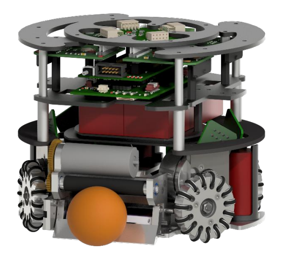
In this ETDP, we will present our new pathfinding algorithm we developed over the course of the last year and successfully used during the RoboCup 2019. We omit any discussion on hardware changes as we are still in the construction phase of the robots described in our last years ETDP [1]. Apart from the new pathfinding algorithm, our success at the RoboCup 2019 can be largely attributed to improvements which we have already discussed in previous ETDPs.

2 Path Planning

In the following section, we describe our new trajectory based path planning algorithm. After a short introduction and problem statement, we describe our trajectory generation method based on an alternative trajectory representation. This representation is refined until it is usable in practice. We then detail the advantages of this method over the more traditional bang-bang trajectories. Finally, we show how to use this trajectory generation method in practice in a complete path planning algorithm.

2.1 Introduction

In order to explain the design decisions that we made regarding our new path planning algorithm, we start by presenting our old approach, its advantages and disadvantages as well as additional constraints.

Until last year, we used two-dimensional Rapidly-exploring Random Trees (RRTs). These are also commonly employed in the league [2,3,4]. We presented a detailed overview of our usage of this approach in [5]. Briefly summarized, the path planning is executed independently for each robot 100 times per second. This limits the accumulated computation time to less than 10 ms for all robots. Every frame, the strategy generates a new set of obstacles to avoid as well as a target position and velocity. The orientation of the robots is controlled separately as the movement direction and orientation of SSL robots are largely independent. It will not be discussed in this paper. The RRT generates a continuous path avoiding all obstacles from the initial robot position to the target. This path generation happens only in position space and does not consider velocities. This path is then processed to be as short as possible. In a second step, a trajectory is constructed close to the generated path taking into account the robots velocity and acceleration limitations. As the construction does not work when the robots current velocity leads away from the desired trajectory, we brake as fast as possible if this case occurs.

While we have used this approach successfully during many RoboCups, it still has some limitations inherent to its design:

• The RRT approach minimizes the length of the path to the target position. For slow velocities, when the robot can brake in a fraction of a second, distance traveled is a good proxy for the time spent driving. When the robots are capable of higher velocities, faster paths can usually be constructed by other means. With higher velocities, traveling longer distances can lead to earlier arrivals when obstacles are present[1].
• As the RRT operates in position space only, all obstacles have to be stationary. Introducing moving obstacles like robots or the ball would require knowledge of the robots position for each given point in time. However, timing information is only computed in the post-processing step once the path is fully assembled.
• We currently employ a velocity controller on our robots, as described in our 2018 ETDP [6]. Moving position control to the robots would allow for better integration of sensor data and more precise driving. However, a position controller on the robots fundamentally clashes with the RRT approach. As the RRT disregards the robots physical limitations, the post-processing is needed for a feasible path. This is repeated every frame and acts as a position controller itself, interacting poorly with a robot based approach.
• The time to the target can not easily be estimated due to the initial velocity of the robot. As the post-processing of the path operates only in one dimension along the path, any initial velocity that strongly deviates from the desired path direction can not properly be accounted for.
• With the RRT, we experienced more collisions than we are comfortable with. To avoid collisions with fast moving robots, we had to drastically enlarge their obstacles in the current driving direction of the robots. For goal shots, we created a large triangular obstacle between both goal posts and the ball. These obstacles hindered our ability to reach the desired target quite often. A solution for this is the usage of moving obstacles whose position is dependent on the current time. These kinds of obstacles are not possible with a 2D RRT. Dynamic Safety Search [7] might present an alternative solution, but we did not implement and test it so far.

All of these limitations can already be overcome with a standard trajectory based path planning using bang-bang trajectories. TIGERs Mannheim showed in their last years ETDP [8] how to apply this to SSL robots. We also give a short introduction to this technique in 2.2.

However, this standard approach does not have all the features of our RRT based path planning, which we would like to keep if possible. Therefore, any new path planning algorithm would have to incorporate the following features:

• If the robot finds itself in an obstacle it must take the shortest or fastest route out of it.
• If the target point itself is inside an obstacle or otherwise not reachable, the robot should drive as close as possible to the target without intersecting any obstacles.
• Our current approach additionally offers to specify a target velocity. It is not mandatory to reach the velocity at the target position. Instead, the velocity is interpreted as a maximum:

Definition 1. Let d be the normalized direction vector the robot reaches the target position with and m the given maximum velocity vector. The maximum scalar velocity at the target position is then the length of the projection of m onto d: m ◦ d.

The path planning algorithm should use this maximum speed to decrease the necessary time to the target if possible. We specify this target velocity when catching a ball or manmarking opponents.

As an alternative method, many of the described RRT disadvantages could be mitigated by using a 4-dimensional RRT, sampling in the joint position-velocity space. However, the necessary computation time would likely become prohibitive for real time applications with quickly changing obstacles.

2.2 Previous Works

As previously mentioned, TIGERs's trajectory based path planning [8] can already solve many of the problems we have been encountering with the RRT. As their approach is quite similar to our proposed version we will provide a short recap.

The path planning is based on the ability to generate feasible trajectories reaching a given position while also adhering to the robots physical limitations. The general approach is to select a set of intermediate positions. Trajectories are generated from the robot to these positions, and then from from the intermediate positions to the target position. The trajectories are then evaluated based on their time and possible collisions with obstacles. The best trajectory is used for controlling the robot.

TIGERs use 2D bang-bang trajectories to compute these feasible trajectories. Bang-bang trajectories are not optimal in respect to the trajectory time, but they provide a computationally feasible approximation. To compute a 2D bang-bang trajectory reaching a desired destination, the typical algorithm separates the problem into two 1D sub-problems in x and y direction. Using a binary search, the distribution of the acceleration and maximum velocity to the directions x and y is found such that the time of both 1D trajectories becomes sufficiently similar, for example within one millisecond [9]. A 1D bang-bang trajectory is either always accelerating, decelerating or is at the maximum allowed velocity. These can be easily computed given the desired distance and acceleration. Therefore, 2D trajectories are typically computed with a target position and acceleration as inputs.

This method has the advantage of being easy, reliable and fast. However, the approach is rather constrained in the ability to match the robots physical acceleration capabilities. Without unreasonable effort, it is only possible to specify exactly one acceleration and exactly one deceleration parameter for the whole trajectory. Additionally, the velocity at the target position is required to be zero.

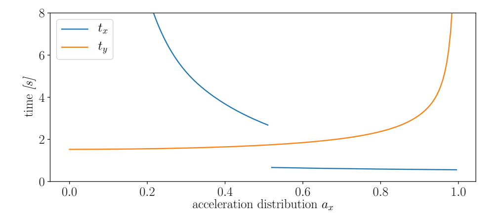
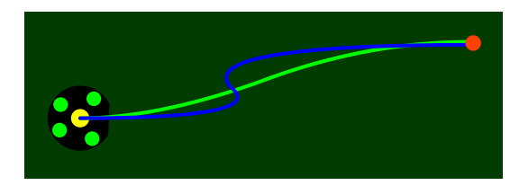
Otherwise, this could lead to discontinuities in the trajectory time. Assume the trajectory generation only to be a function mapping acceleration to the time for a given target state in one dimension. This function is discontinuous when introducing target velocities. Therefore, there exist scenarios without an acceleration distribution $a^x$ for which both one-dimensional functions yield the same value. The existence of such a value $a^x$ is necessary to construct a valid 2D trajectory. Figure 2 shows an example without a valid intersection.

2.3 Trajectory Generation

Without loss of generality, we will assume the initial position of the trajectory to be at (0,0) in the following section. The target velocity is required to be zero. Non-zero target velocities will be discussed in a later section. The initial velocity at the beginning of the trajectory will be denoted by $v^i$.

The main contribution of this ETDP is the introduction of an alternative trajectory generation method. It combines both the advantages of our RRT approach as well as those of TIGERs's solution [8]. As previously explained, the standard method of generating 1D bang-bang trajectories uses the desired distance and acceleration as inputs. However, there are also alternative ways to define and compute these trajectories. It is sufficient to know two of the three parameters time, distance and acceleration to uniquely define a 1D bang-bang trajectory. Our proposed method uses the time and acceleration.

Our 2D bang-bang trajectories are therefore parameterized by a given time and acceleration distribution $a_x$. In order to simplify the presentation, this section uses an acceleration a=1. This simplifies the acceleration in x direction to $a_x$. As usual, the maximum acceleration should be used whenever possible, the acceleration $a_y$ in y direction can be calculated using

$$\sqrt{a_x^2 + a_y^2} = 1 \quad (1)$$

As the time is already given as a parameter, it is no longer necessary to use bisection to find a valid trajectory.

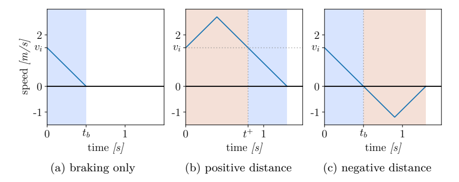
Using just time and acceleration distribution as parameters, it is not possible to reach every position on the field. For each dimension, the input time can be divided into two parts, the time necessary to fully brake given the acceleration in that dimension $t_b$ and some additional time. We define these additional times as the possibly different values $t_x^+$ and $t_y^+$ in the x and y dimensions respectively. To be able to reach every point on the field, it must be possible to use $t_x^+$ and $t_{\eta}^{+}$ to drive both a positive and negative additional distance. See Figure 3 for three velocity/time diagrams of different bang-bang trajectories demonstrating this additional time. Two additional bits of information are necessary to specify the type (positive/negative) of this additional distance for each direction. Since equation 1 describes a circle, we can substitute the acceleration distribution with an angle. This results in a trajectory generation function that takes time and an angle as inputs. From this point onward, t and $\gamma$ will denote these parameters for the trajectory generation. The 1D acceleration can now be computed as $a_x = |\sin(\gamma)|$ and $a_y = |\cos(\gamma)|$. The sign of the trigonometric functions define whether the trajectory should travel a positive or negative distance in the respective direction. Note that the angle does not precisely correspond to the actual direction the trajectory will lead to, this issue will be addressed later.

The trajectory generation still has the problem that some inputs do not correspond to an actual trajectory. There are two cases for which the inputs are invalid:

1. It is not possible to fully brake if the given time t is too low: $t < \frac{|v^i|}{a}$. This case can be handled easily by avoiding input values smaller than the minimum braking time $\frac{|v^i|}{a}$ or always adding the minimum braking time to t.
2. It is possible to fully brake in the given time, but not with the acceleration distribution specified by $\gamma$. This is true for $\frac{|v_x^i|}{a_x} > t$ or $\frac{|v_y^i|}{a_y} > t$. For any given t, there exist four of these invalid regions of $\gamma$, around $0, \pi/2, \pi$ and $3/2\pi$.

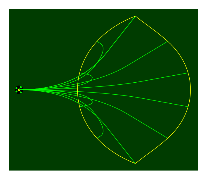
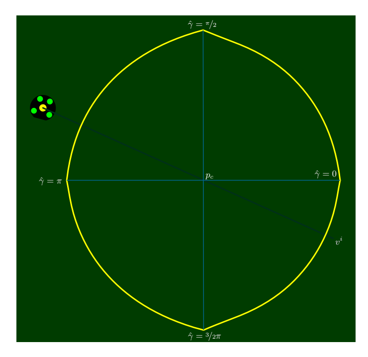
A convenient way to handle these cases is to transform $\gamma$ such that the invalid regions from point 2 disappear. The size of the regions around 0 and $\pi$ can be computed by finding $\gamma_x$ such that $\frac{|v_x^i|}{a \cdot |\sin(\gamma_x)|} = t$. This is solved by $|\gamma_x| = \sin^{-1}(\frac{v_x^i}{t \cdot a})$. The equivalent computation can then be performed in y direction with $\gamma_y$. Eliminating the invalid regions can be visualized as cutting the corresponding angles out of a circle and re-assembling the remaining parts to a smaller, roughly spherical, shape. A visualization of this process is shown in Figure 4. The new angle without invalid regions is then defined as $\hat{\gamma}$. To compute $\gamma$ from $\hat{\gamma}$, we first check in which quadrant $\hat{\gamma}$ lies. We then linearly interpolate the $\hat{\gamma}$ to the corresponding valid segment of $\gamma$.

This transformation is not just convenient for having a total function. Additionally, the space of generated trajectories is continuous, as the trajectories for $\gamma = \gamma^x$ and $\gamma = -\gamma^x$ are the same. We show this fact for the invalid region around 0, the other regions work analogously. The trajectories in y direction for $\gamma^x$ and $-\gamma^x$ are the same since $\cos(\gamma x) = \cos(-\gamma x)$. This is contrasted by the x direction, where $\sin(\gamma x) = -\sin(-\gamma x)$ holds. While the resulting sign value differs in the x direction, it is not used, as by definition $\gamma^x$ is the angle such that the trajectory only consists of braking to a velocity of zero. Therefore, the sign is only important if the additional time $t^+_x$ is nonzero. As a result, the trajectories at $\gamma^x$ and $-\gamma^x$ are exactly the same.

To illustrate the continuity of the trajectories for a given time, Figure 5 shows the target position of all trajectories reachable in a given time in yellow as well as selected trajectories in green.

2.3 Trajectory Generation (continued)

Trajectories Reaching a Given Position The last section showed that the trajectory generation parameterized by time and angle can be well defined and continuous. Up until this point, we discussed trajectories traveling to unspecified positions. In contrast, path planning algorithms require trajectories traveling exactly to a specified position. In order to arrive at a given position, we need to determine the corresponding values of t and $\hat{\gamma}$. The required search algorithm operates in two dimensions and is therefore too complex to use binary search.

Instead, we propose an alternative iterative algorithm. As initial trajectory parameters, we compute an approximate time and angle. The algorithm will find the correct solution regardless of the choice of initial parameters, but a better heuristic will speed up the search. The time and angle are then repeatedly updated until either a trajectory with the desired target position is found or too many iterations have passed. The second case rarely happens but is necessary as a fail-safe.

To improve the search algorithm, we introduce additional geometric interpretation of the angle. First, consider the following fact: for a fixed time, the final positions for the trajectories at $\hat{\gamma} = 0$ and $\hat{\gamma} = \pi$ have the same x coordinate as $\sin(\gamma x) = \sin(\pi - \gamma x)$. A similar fact can be observed for the y coordinate at $\hat{\gamma} = \pi/2$ and $3/2\pi$. We define $p^c$ as the point at these x and y coordinates. Figure 6 shows this point inside the shape of all positions reachable in a fixed time. While it may not exactly be at the geometric center, it is fairly close. Geometric angles of final positions of trajectories can now be computed in reference to $p^c$. By construction, the geometric angles at $\hat{\gamma} = 0, \pi/2, \pi, 3/2\pi$ exactly correspond to $\hat{\gamma}$. As the final positions vary continuously and roughly uniformly, the angles in between also approximately match their respective geometric angles. Measurements shows that the average difference between these two angles for realistic scenarios is low. The input angle can therefore be used as an approximation for the target position angle. This allows for better heuristics for updating the input angle in the iterative algorithm.

$p^c$ could be computed by generating two trajectories with input angles 0 and $\pi/2$. This expensive computation can be avoided by realizing that $p^c$ can be computed as $v^i \cdot \frac{t}{2}$ with $v^i$ being the initial velocity. This holds for all t, independent of a.

For updating the time and angle, we use the following heuristics: Let $p_t$ be the desired target position and $p_f$ the final position produced by the current time $t_i$ and angle $\gamma_i$. We update $t_i$ as

$$t_{i+1} = t_i + (|p_t - p_c| - |p_f - p_c|) \cdot f \cdot h(t_i, \gamma_i)$$ (2)

where f is the update strength. We modify f accordingly to compensate overshooting the distance. h is a heuristic function used to speed up the search (see our open source code for more detail). The angle is updated in a similar fashion using the geometric angle between $p_t$, $p_c$ and $p_f$.

Using these heuristics like these for updating the time and angle, this search terminates in surprisingly few steps, depending on the target precision. If the trajectory does not exactly reach the target position, it can be slightly stretched in such a way that it does so precisely. This slightly distorts the acceleration at different points on the trajectory, but the distortion effect is negligible as long as the distance traveled on the trajectory is significantly longer than the position error. As a result, a higher precision is necessary for shorter distances than for longer ones. We usually use a target precision of one centimeter for longer trajectories.

To analyze the efficiency of our search algorithm, we ran the search for varying inputs. For different precisions, we tested random initial velocities and distances. The average number of iterations for a trajectory was recorded and can be seen in Table 1. It can be seen that the necessary number of iterations is not significantly higher than the number typically used for the classical binary search algorithm (around 10). As the work done in each iteration is similar, the performance of our proposed algorithm is on-par with the previous one.

2.3 Trajectory Generation (continued 2)

Advantages While we have established that our algorithm can compute trajectories quickly and reliably, we have not yet detailed the advantages over the classical approach given the increased complexity.

The first advantage is that target velocities can be used. Different semantics for target velocities are possible, including:

• No target velocity: The velocity at the target position must be zero. This is the option used in most approaches that were discussed so far.
• Exact target velocity: The generated trajectory must have the exact target velocity specified by the input. This should not be used for the target position of the whole trajectory, as slight variations in the robot speed or position will result in very different trajectories. See Figure 7 as an example of this phenomenon. However, exact target velocities can be used for intermediate trajectories, as the position and velocity of intermediate points can be updated every frame.
• Maximum target velocity: This is the semantic we used in our RRT based path planning algorithm, using the projection of the target velocity on the trajectory direction at the target position, as stated in Definition 1.

Other semantics are possible in principle but we found the listed ones to be sufficient.

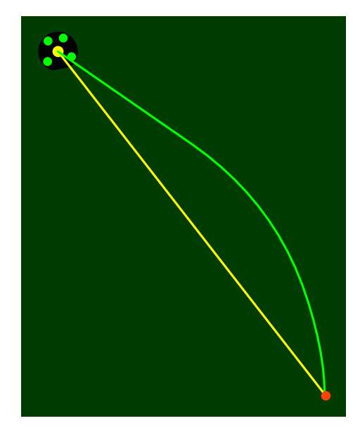
All of these options can be achieved with the proposed algorithm. The 1D bang-bang trajectory generation can be easily modified to include these features. The space of trajectories will stay continuous and the search algorithm can remain basically unchanged. While all formulas like for example the size of the invalid angle segments have to be slightly adjusted to include the target velocity, these changes are trivial. Figure 8 shows an example of a trajectory with and without a maximum target velocity. In this case, the target velocity is used to decrease the necessary time to the target. While the regular straight trajectory takes around 1.6 seconds, the trajectory using the target velocity pointing down only needs 1.4 seconds. If the target velocity pointed up, the trajectories would be the same, as no speedup can be achieved.

The second advantage is that we can match the acceleration profile to that of real robots. Real SSL robots have a varying maximum possible acceleration at different velocities and orientations [9]. While the minimum possible acceleration of any robot configuration can be used, this may leave a lot of acceleration potential unused.

We propose to adapt the trajectory to the actual acceleration profile as follows. After generating a trajectory with a time and angle inside the search algorithm, a second pass over the trajectory is performed. The acceleration at all points along the trajectory is modified to match the robots acceleration profile. Changing the acceleration will modify the resulting distance traveled as well as the trajectory time. Since the target position is not a parameter of the trajectory but rather searched for in the surrounding search algorithm, this modification of the distance is compensated by the search algorithm. We propose two methods to adapt the acceleration. The first method subdivides the trajectory into short time intervals. A constant acceleration is assumed for these intervals to compute their distances. A second approach takes all segments with constant acceleration in both dimensions and analytically solves the matching integral over the acceleration to obtain the segments distance. The first approach will always work but consume significantly more computational power, while the second one may not always be feasible.

2.3 Trajectory Generation (continued 3)

2.3 Trajectory Generation (continued 4)

2.3 Trajectory Generation (continued 5)

2.4 Sampling Strategy

TIGERs described a strategy for sampling trajectories to find a valid path to the target while avoiding obstacles [8]. Their approach is fully compatible with the trajectory generation described in this paper, although it might not make full use of its potential. As target velocities are possible with our trajectory generation, we use an alternative sampling strategy. It operates in the four dimension space spanned by exact target velocity in two dimensions, time and angle. We heuristically select a number of points from this space and generate two trajectories. The first trajectory can be computed with the target velocity, time and angle. It travels from the robot to some unspecified position on the field. The second trajectory then picks up from there and travels to the target position. While this approach needs to search for paths in a higher dimension than the approach by [8], it also has the potential for trajectories of a higher complexity. As an example for this complexity, Figure 9 shows the optimal trajectories around a defense area with our approach compared to [8]. The trajectory sampling method employed by [8] generates a far longer path with a duration of 3.12 seconds. Our proposed sampling method generates a trajectory far closer to the defense area which would take around 2.65 seconds to drive. However, this difference might not be too relevant in practice, as such situations do not occur too often in real SSL games. In addition, as soon as the robot reaches the next corner of the defense area, the sampling approach of [8] will find a more reasonable path as a lower trajectory complexity is necessary. This can lead to similar drive times for both algorithms. The major advantage of our approach lies in the earlier knowledge of the correct arrival time.

3 Conclusion

In this ETDP we presented our new path planning algorithm with capabilities like target velocities and accelerations depending on robot configuration. This algorithm was of great help during the RoboCup in Sydney. However, some challenges remain unsolved. While the path planning algorithm works as intended, the choice of obstacles for robots and the ball has a strong influence on the resulting trajectory quality. This is especially true for opponent robots, which can not easily be predicted. For example, collisions with opponent robots are sometimes hard to avoid when their obstacles are not large enough to compensate for unpredictable changes in speed or direction.

The new algorithm also allows us to test approaches that were previously impossible. We plan on testing a ball interception method embedded inside the path planning algorithm, essentially using a moving target position. This could present a novel application of this type of path planning algorithms.

References

1. Engelhardt, T., Heineken, T., Kühn, T., Lindner, J., Schmidt, M., Schofer, F., Seifert, C., Stadler, M., Wegmann, L., Wendler, A.: ER-Force 2019 Extended Team Description Paper. (2019)
2. Yoshimoto, T., Horii, T., Mizutani, S., Iwauchi, Y., Zenji, S.: OP-AmP 2019 Extended Team Discription Paper
3. Huang, Z., Chen, L., Li, J., Wang, Y., Chen, Z., Wen, L., Gu, J., Hu, P., Xiong, R.: ZJUNlict Extended Team Description Paper for RoboCup 2019. (2019)
4. Mirahy, B., Machado, É., Moreira, E., Azevedo, F., da Silva, J., Luciano, J., Santos, M., Máximo, M., Lima, R., Linhares, R., et al.: ITAndroids Small Size Soccer Team Description 2019. (2019)
5. Eischer, M., Blank, P., Danzer, A., Hauck, A., Hoffmann, M., Reck, B., Eskofier, B.M.: ER-Force Extended Team Description Paper RoboCup 2015. (2015)
6. Lobmeier, C., Burk, D., Wendler, A., Eskofier, B.M.: ER-Force Extended Team Description Paper RoboCup 2018. (2018)
7. Bruce, J.R.: Real-time motion planning and safe navigation in dynamic multi-robot environments. Technical report, Carnegie-Mellon Univ Pittsburgh PA school of computer science (2006)
8. Ommer, N., Ryll, A., Geiger, M.: TIGERs Mannheim Extended Team Description for RoboCup 2019. (2019)
9. Purwin, O., D'Andrea, R.: Trajectory generation for four wheeled omnidirectional vehicles. In: Proceedings of the 2005, American Control Conference, 2005., IEEE (2005) 4979–4984