RoboFEI 2020 Team Description Paper
Leonardo da S. Costa, Wesley de S. Motta, Danilo Pilotto, Guilherme L. Pauli, João V. L. Aguiar, Gabriel M. Schiavetto, Bruno Bollos Correa, Mateus Mariano Lucatelli, Marcos A. P. Laureano, Reinaldo A. C. Bianchi, Plínio Thomaz Aquino Junior, Flavio Tonidandel
Robotics and Artificial Intelligence Laboratory Centro Universitário da FEI, São Bernardo do Campo, Brazil
Abstract This paper presents the current state of the RoboFEI Small Size League team as it stands for RoboCup International Small Size League competition 2020, in Bordeaux, France. The paper contains descriptions of the new electronic board design, a new modeling technique for the robots as well as a new position controller.
Introduction
For RoboCup 2020, the RoboFEI team intends to use mostly the same electronics and mechanical design that have been used over the last years. However, there are plans to test the new robot design, the mechanics are already described in last year TDP [8].
Some significant advances were made in our software, the improvements were verified in the XVIII Latin American Robotics Competition (LARC), which resulted in our seventh first place trophy. The objective now is to improve furthermore the software system and start replacing our current robots. With our researches, we hope to bring innovations and new ideas for the community.
Electronics
Restructuring the electronic boards using a modular structure has been the goal since RoboCup 2019. Each function will be arranged on a smaller board and all blocks will communicate over connections through a main board. This change aims to facilitate the maintenance of the robot. When identifying a problem, the faulty module will be replaced and separated for further analysis.
The first prototypes are being produced for RoboCup 2020. As soon as the new boards work properly, the old ones should be quickly replaced.
Modular Structure
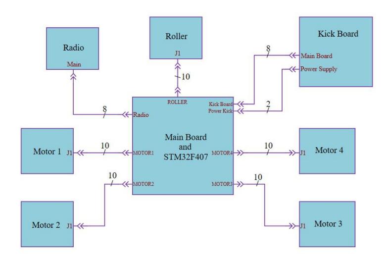
Compared to the current structure, where the whole electronics are divided into a main, kick and radio boards, in the new structure there are nine modules. These modules consists of five motor, one kick, one main, one radio and one STM32F407 Discovery boards. The block diagram representing these modules can be seen on Figure 1.
Kick Board
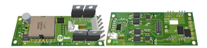
The new kick board works with the Flyback topology based on the IC LT3751, the choice of this controller model was due to the possibility of checking the input voltage and defining an operating range, making it safer for the batteries. The system uses a 4000µF/200V capacitor. For the kick activation, it uses the IXFA56N30X3 MOSFET, which supports 300V and 56A. The board can control up to three solenoids.
For the capacitor, solenoids, battery and main board communication we use the connectors WM18823, WM4624, WM4300 and M20-9980445, respectively.
The board model can be seen on Figure 2.
Motor Board
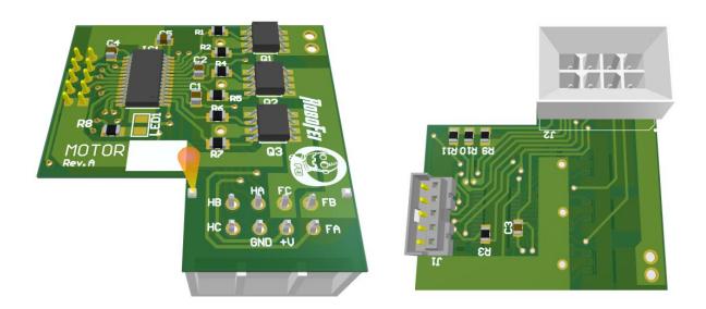
Composed of the IC A4915 in conjunction with the IRF8313TRPBF MOSFET, the board receives a PWM signal for the motor and is responsible for controlling its speed using the input and feedback from all hall sensors.
The connector of choice for connecting the motor and main boards is the SAM11451 due to its robustness, which will be verified in the first prototypes.
The board model can be seen on Figure 3.
Main Board
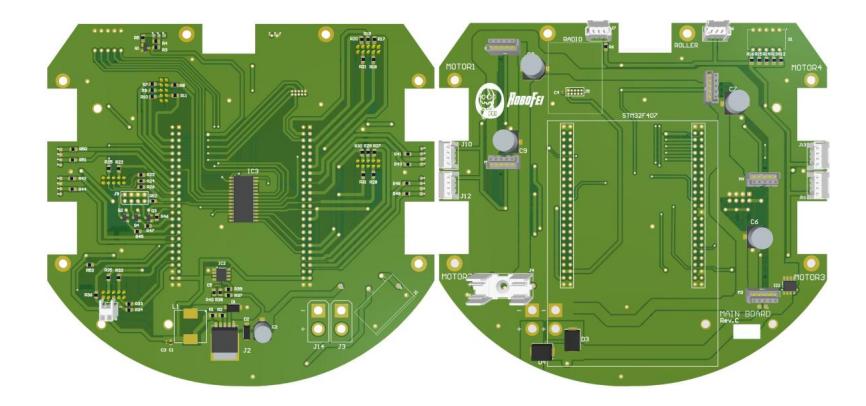
Responsible for connecting all modules and performing the power and regulation necessary for the operation of each board and peripherals. The power will be carried through two 14, 8V batteries with a capacity of 1300mAh for better arrangement inside the robot. The supply voltage goes through a 5V buck regulator that will be distributed throughout the board.
To avoid connection issues with the encoder connectors, which were very present in our current main board, we are using the WM18921 connectors. For the battery connection we used the XT60.
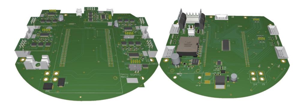
The board model can be seen on Figure 4.
Assembly
In Figure 5 there is the assembly of all modules developed by the team. The radio and STM32 boards aren't placed in the 3D model, but, their places and connectors are being considered. The radio board is the nRF24L01, which is the same from last years.
With these changes, we are looking for a structure that will simplify design developments for a new control board that will make it easier to make improvements, such as: achieve a better movement control with the new motor drivers, faster charging and higher durability of the kick board, making future improvements in electronics easier, since the structure is divided into several boards, in case of changes in one module the others will still work properly.
By analyzing previous (E)TDP from other teams [13,10,3], it is noticeable that a few years ago there was a majority of teams using FPGAs as the main controller of the robot. However, nowadays, there are a lot of teams using STM micro controllers instead.
Due to the great peripherals that the STM32 micro controller has, such as timers that can be configured to read the encoders, we've decided to migrate to it. That way, the development of a new firmware should be fairly easier than using a FPGA.
In a future version of our main board we plan to stop using the STM32F407 Discovery board and use only the STM32 chip, that way the board layout should be greatly simplified.
System Identification
In order to project a good controller it is important to have a good model of the plant which will be controlled. Therefore, some knowledge about the plant parameters is necessary, e.g. friction coefficients. However, some of the parameters can be hard to measure, thus, complicating the task of accurately modeling the plant using classical laws of physics. To avoid this problem there is a modeling technique called system identification, which consists of estimating/identifying the plant model using data from its input and output [6].
Plant excitation
As already said, to identify a certain model, it is necessary to have data from the input and output of the plant. Note that this data need to be as much informative about the plant behavior as possible. The identified model will only be able to reproduce behaviors that were captured by the data used in the estimation, thus, the importance of the data quality.
In order to gather informative data that result in a good model there are some commonly used signals which can be used. Those signals are: Pseudo Random Binary Signal (PRBS), Generalized Binary Noise (GBN) and Step function.
PRBS The PRBS signal is commonly used in system identification for linear systems, it is a deterministic signal with properties of a random signal [11]. Due to its white-noise like properties, this kind of signal is capable of exciting the dynamics of the plant in various frequencies. It can be generated using a Linear Feedback Shift Register (LFSR) [9], and is parameterized by the number of bits n in the shift register and the switching time Ts.
GBN The GBN is a stochastic binary signal which switches between two fixed levels [12]. At every time sample it has a probability p of switching to another level. This probability has to be correctly determined for each plant, [12] proposes some guidelines that can be used to choose a good value for p.
Step Signal Although it is considered as a poor signal, i.e. doesn't provide much information about the system, it can be used when identifying simple systems. According to [12], it is better to use a step signal than a badly parameterized binary noise based signal. In the control area this is a widely used signal, most of the system parameters are acquired using the step response experiment [7].
Model formats
After choosing an input signal, it is necessary to pick a format for the model to be identified, there are several mathematical formats, the most common are: Transfer functions, Space State and Polynomials.
The model format is also an important choice to make, depending on the type of plant some models can adapt better than others. When dealing with linear Single Input Single Output (SISO) systems, a common choice is the transfer function [7].
Considerations About the Robot
Since the robots used in the SSL are omni-directional, its three axis are independent, thus, the whole robot can be considered as three separate SISO systems.
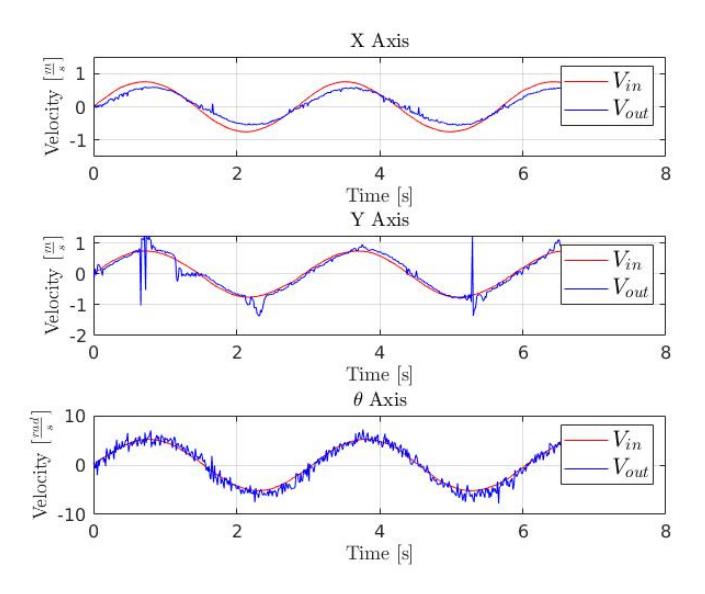
By using the harmonic analysis method [5] it is possible to see that the X, Y and θ axis can be considered as linear, since, apart from the noise and some attenuation, there is no presence of other harmonics than the one present in the input, this can be seen on Figure 6, the signals used were Vi(t) = 0.75∗sin(t), i = x, y [SI] and Vθ(t) = 5.4 ∗ sin(t) [SI]. This analysis can also be verified by using the Discrete Fourier Transform, if the system is linear, the DFT of the input and output should be practically the same.
There is a considerable noise present in the data collected for the Y and θ axis presented in Figure 6. This happens because these velocities were calculated based on the raw position of the robot.
Figure 6 also shows a small phase shift for the X axis, a possible cause for this is the influence of the angle that the robot is facing (θ). During the tests it was noticed that depending on the value of θ, when working in a open loop, there may be a slight phase shift and even some attenuation for the X axis. This effect doesn't seem to be noticeable in the Y axis.
Identifying the Models
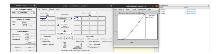
To actually do the identification of the models, the System Identification Toolbox from MATLAB was used. The toolbox interface can be seen on Figure 7. The first step is to import the working data. After importing the data, in the 'Estimate →' option it is possible to choose which model it will estimate, e.g. transfer function model, and then the model output can be seen by clicking on the 'Model output' checkbox.
Being a linear SISO system facilitates a lot of the process of identifying the models of our robots, as well as the controller project. Therefore, the model format of choice was the transfer function, due to the ease of applying classical control theory on it.
Given that the purpose of the model is to design a position controller for our robots, the model input will be the velocities Vx, Vy, and Vθ, which are the velocities that the robot must move in the X, Y and θ axis in the field reference. The model output will be the field position of the robot in each axis.
Data Acquisition
As said earlier, the quality of the working data is crucial for a good model estimation. One thing that needs to be assured when gathering the data is the sampling interval, since the models will likely be used in its discrete form, the sampling interval must be constant. Given that the actual control loop runs at a 15ms interval, it will be the sampling time used.
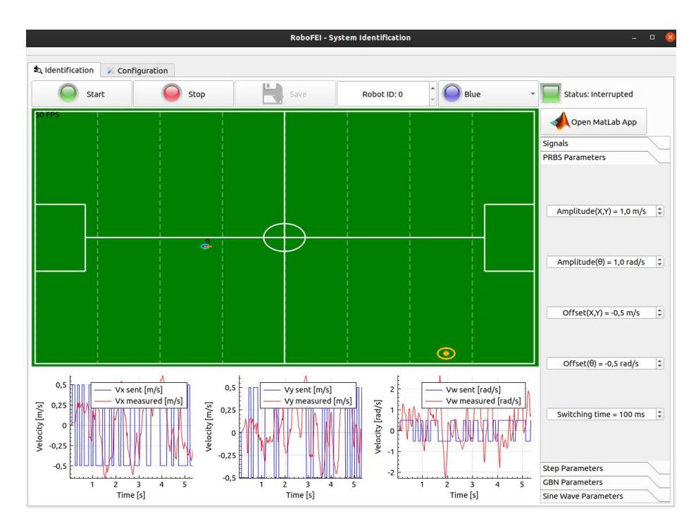
To guarantee that the signals will be sent and measured in the right interval, a dedicated software was built. Basically it is responsible for generating any of the signals commonly used in the process of identification, i.e. PRBS, GBN, Step and Sine, sending these signals to the robots and measuring the position of the robot. In Figure 8 it is possible to see the software interface, at the bottom left there are some graphs to see the signal being sent, in the top right there are the parameters of each type of signal. In the future, the software will be integrated with MATLAB to make it easier to generate the models.
Input Signal
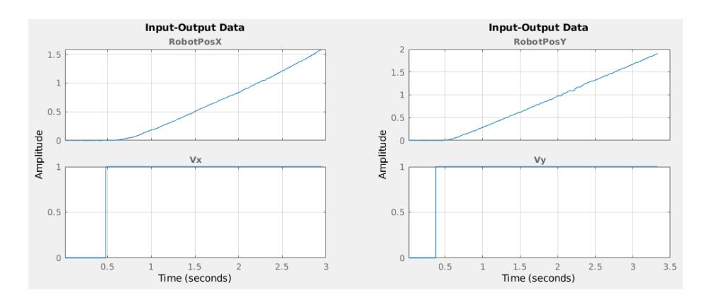
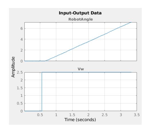
Since the model format is a transfer function, the step response experiment was used to collect the data needed. Some previous experiments have shown that it is possible to estimate good models using this experiment.
The measured data can be seen of Figures 9 and 10. Note that this is an open loop experiment, therefore, it is expected that the X,Y and θ values tend towards infinity.
Models
When using the tools that MATLAB offers to identify transfer function models it is necessary to set how many poles and zeros the transfer function must have. By doing some experiments it was discovered that the robot behavior can be accurately modeled using two poles and none zeros, and in some cases two poles and one zero.
Using the data shown in Section 4.2 the discrete transfer functions for the X, Y and θ axis were identified and can be seen on Equations (1), (2) and (3).
$$\frac{P_x(z)}{V_x(z)} = \frac{0.0003494}{z^2 - 1.97z + 0.97}$$
$$\frac{P_y(z)}{V_y(z)} = \frac{0.0006378}{z^2 - 1.94z + 0.9399}$$
$$\frac{P_{\theta}(z)}{V_{\theta}(z)} = \frac{0.001623}{z^2 - 1.901z + 0.9009}$$
The compare command outputs a graph which show how close the model output is to the given data. On Figures 11 and 12 it is possible to see that all models have more than 97% of accuracy when representing the robot.
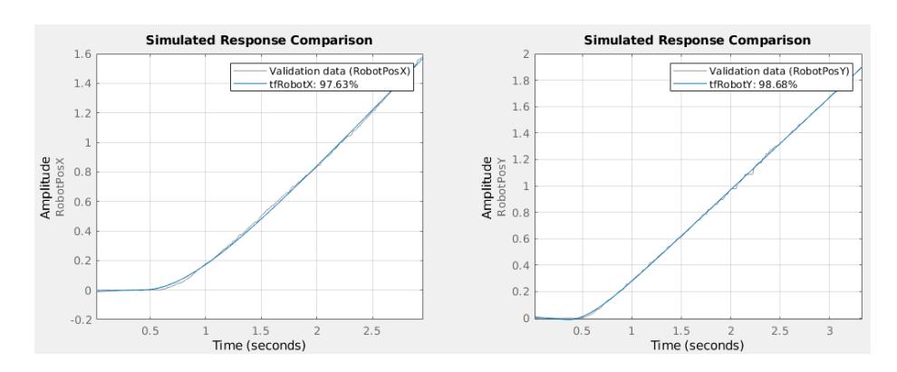
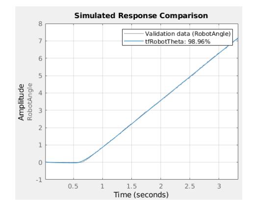
These results show that the models can accurately represent the behavior of the robot, therefore, it is now possible to design the position controller.
Position Controller
By having the models of the robot, it is possible to design the position controller that gets the robots to its destiny.
The controller of choice is the classic Proportional Integrative Derivative (PID)[7]. It is a very robust controller and can be easily tuned using MATLAB and its PID Tuner Toolbox.
Tunning the Controller
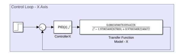
The first step to tune the controllers is to create the block diagrams in Simulink, the result for the X axis can be seen on Figure 13. For Y and θ axis it is exactly the same diagram, except for the transfer function model values.
The windup effect is caused by an overflow of the integrator in the loop. It usually happens when the plant saturates for an extended period of time and the integrator continues to integrate the error [4]. Therefore, it is important to have some kind of anti-windup method.
The PID block offers two anti-windup methods. The one chosen for this application is the clamping method. It is one type of conditional integration and works by stopping the integrator once the system meets a certain condition [2,1].
The saturation limits must also be defined, the values chosen were ±1.75 m/s, which is the highest speed the robots can drive without too much slipping. For the angular velocity the limits are ±6.25 rad/s.
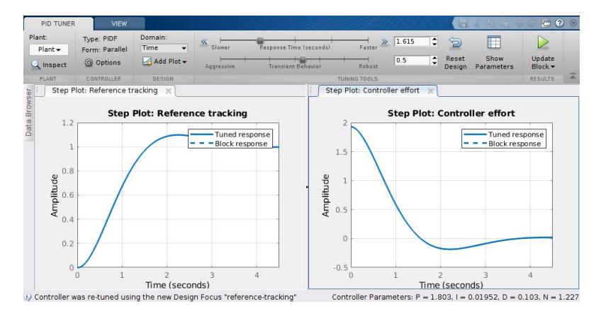
Using the 'Tune' button in the PID block it is possible to tune the controller. The PID Tuner interface can be seen on Figure 14. In this example, the tuned system performance parameters can be seen on Table 1.
The controller block can be updated using the 'Update Block' button.
System performance parameters.
| Rise time [s] | Settling time [s] | Overshoot [%] | |
|---|---|---|---|
| X | 1.05 | 3.48 | 9.8 |
| Y | 0.795 | 2.19 | 3.84 |
| θ | 0.165 | 0.525 | 7.03 |
Using the two sliders on the top of the window (Tuning Tools upper section) it is possible to adjust the transient response of the system, the effects of the changes can be seen on the step plot. The design focus can be changed to 'Reference tracking' (Controller upper section). This option helps to diminish the overshoot.
During a few experiments, the controllers that behaved better on the actual robots were the ones that had a smooth control effort, therefore, adding its plot is helpful (Design upper section) in the tuning process.
Deploying the Controller
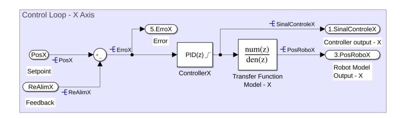
After tuning the controllers for all axes it is time to implement them in the strategy software. By doing a few adjustments to the block diagram in Simulink it is possible to export it to C++ code using the Embedded Coder feature. The final block diagram can be seen on Figure 15.
Basically, all that needs to be done is to add the inputs/outputs blocks to the control loop, e.g. set-point position, feedback, output to the system. This step is important because this is how MATLAB will know what variables must be added to interact with the generated code.
Results
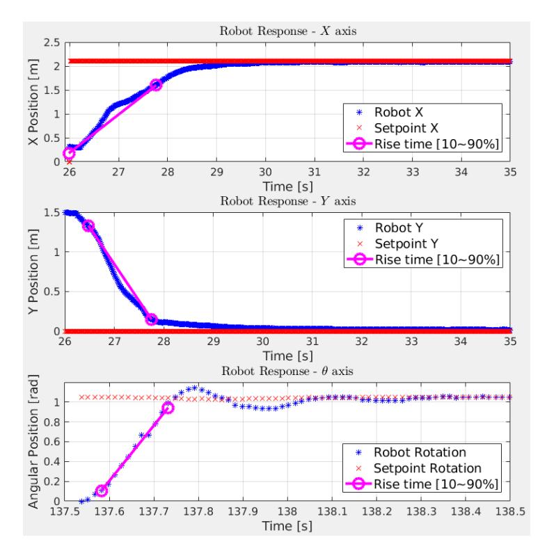
The new controller showed some reasonably good results and the improvements in the speed and precision of the robot are visibly noticeable. The step response for all axes can be seen on Figure 16.
The measured system parameters can be seen on Table 2.
Note that for the θ axis, the variation on the system parameters is smaller than for the X and Y axes. During θ test there wasn't as much slipping as there was for the other two, which clearly resulted in it being closer to the theoretical parameters.
At the beginning of the X and Y tests there as a slight slipping of the wheels, which most likely resulted in its parameters having a higher deviation from the theoretical ones. Slipping is an example on non-linearity that may happen in the system. However, it can be fixed by doing a few improvements in the control loop of the wheels itself, e.g. a better handling of its acceleration, which is currently absent.
Measured system performance parameters.
| Rise time [s] | Settling time [s] | Overshoot [%] | |
|---|---|---|---|
| X | 1.785 | 3.299 | 0 |
| Y | 1.275 | 3.210 | 0 |
| θ | 0.150 | 0.735 | 9.287 |
Acknowledgements
We would like to thank, in advance, the Small Size League Committee, for the consideration of our material. We would like also to immensely thank the staff of Centro Universitário FEI, for all the help we always received from them.
References
- Åström, K.J., Hägglund, T., Astrom, K.J.: Advanced PID control, vol. 461. ISA-The Instrumentation, Systems, and Automation Society Research Triangle. (2006)
- Bohn, C., Atherton, D.: An analysis package comparing pid anti-windup strategies. IEEE Control Systems Magazine 15(2), 34–40 (1995)
- Chen, L., Jin, L., Lon, C.W., Wen, L., Gu, J., Li, J., Fang, T., Xiong, R.: Zjunlict extended team description paper for robocup 2018. RoboCup Wiki as extended team description of ZJUNlict, Montreal, Canada, accessed March 6, 2019 (2018)
- Guzmán, J.L., Åström, K.J., Dormido, S., Hägglund, T., Piguet, Y.: Interactive learning modules for pid control. IFAC Proceedings Volumes 39(6), 7–12 (2006)
- Hosseini, S.M., Johansen, T.A., Fatehi, A.: Comparison of nonlinearity measures based on time series analysis for nonlinearity detection (2011)
- Ljung, L.: System identification. In: Signal analysis and prediction, pp. 163–173. Springer (1998)
- Ogata, K., Yang, Y.: Modern control engineering, vol. 4. Prentice hall India (2002)
- de Oliveira, G.P., Alves, V.M., Pilotto, D., de S. Motta, W., da S. Costa, L., Pauli, G.L., et al.: Robofei 2019 team description paper. . (2019)
- Panda, A.K., Rajput, P., Shukla, B.: Fpga implementation of 8, 16 and 32 bit lfsr with maximum length feedback polynomial using vhdl. In: 2012 International Conference on Communication Systems and Network Technologies. pp. 769–773. IEEE (2012)
- Ryll, A., Ommer, N., Geiger, M., Jauer, M., Theis, J.: Tigers mannheim
- Tangirala, A.K.: Principles of system identification: theory and practice. Crc Press (2014)
- Tulleken, H.J.: Generalized binary noise test-signal concept for improved identification-experiment design. Automatica 26(1), 37–49 (1990)
- Vedder, K., Schneeweiss, E., Rabiee, S., Nashed, S., Lane, S., Holtz, J., Biswas, J., Balaban, D.: Umass minutebots 2017 team description paper (2017)