KIKS Extended Team Description for RoboCup 2022
Ryoma Mitsuoka, Yusei Naito, Yasutaka Tsuruta, Daichi Miyajima, Kosei Naito, Hironobu Suzuki, Ryuto Tanaka, Hayato Mitsuda, Yota Dori, Toko Sugiura
National Institute of Technology, Toyota College, 2-1 Eisei-cho, Toyota, Aichi 471-8525, Japan
www.ee.toyota-ct.ac.jp/~sugi/RoboCup.html
Abstract This paper presents details of the robot and software system of KIKS, a SSL team intending to participate in RoboCup 2022 in Thailand. In this ETDP, we will focus on hardware design for dribbler and electrical circuit board. Weaknesses of previous generations are outlined and improvements to rise above them are discussed including the software upgrading. Furthermore, the implementation of the on-board camera to utilize to the Vision-Blackout is outlined.
1 Introduction
KIKS has continuously developed the higher-performance hardware and smart AI system. In this year, we worked actively to upgrading and expanding of ball control performance for hardware, especially, effective improvements in dribbling system. The development of new circuit board using Jetson Nano and the implementation of the on-board camera to utilize to the Vision-Blackout is also described. In software, we checked in detail for motor control parameters of the robot, and improved AI system using neural networks and Monte Carlo Tree Search (MCTS) for decision-making algorithm introduced two years ago.
2 Mechanical system
In the RoboCup Small Size League, the dribbling system is very important to realize the strategy of AI, recently. We proposed two ideas for dribbling system in ETDP2020[1]. Both of them, however, the interfere with the other units around structure and could not result easily changed. Therefore, in this section we introduce a simple dribbling system that can increase the ball-holding power without major modifications.
2.1 Dribbler
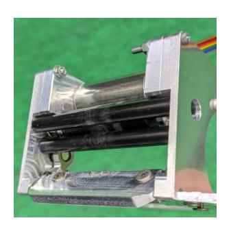
One of the dribbling-mechanisms proposed at ETDP2020[1] was to use two dribbling-rollers shown in Fig.1, and the other one was to make the anglechangeable dribbler unit shown in Fig.2. In the former, however, the power wheel (which transmit the rotation and the torque from motor to the rollers) could not enough transmit the torque to the rollers. As the result, it was found that it could not enough transmit the rotation to the ball. The latter was able to hold the ball, but it interfered with others units. It was necessary to redesign the structure. So, based on above results, we examined more simple and effective structure.
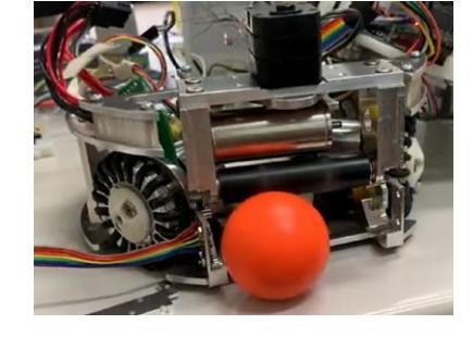
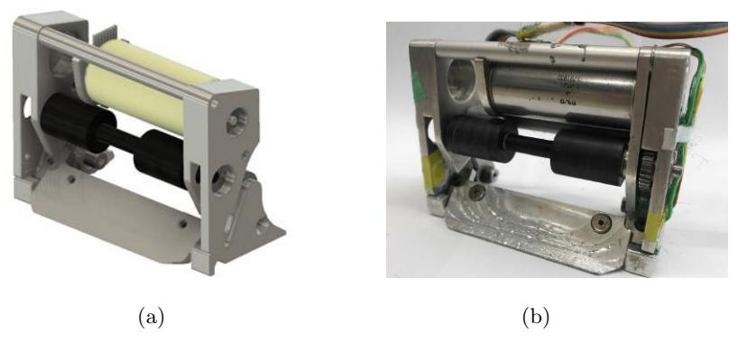
The idea is to divide the dribbler to two parts. Figure 3 show the (a)CAD image and (b)photo of proposed dribbler, respectively. The dribbler has a diameter of 15 mm and a central divided width of 21 mm. It is used polyurethane (hardness shore A50) as the roller material. For the dribbling motor we use maxon ♯ 283860 with gear ratio 1.4. The height from the carpet to dribbler's metal axis (diameter 4 mm) is about 36 mm.
In this case, it cover only about 16% of the ball (not violating the 20% rule even in shock-absorbing mechanism) when we look down the robot from straight above. This idea was referred to the technique used by many teams in the RoboCup Soccer Junior League. This structure has the following merits.
- It can be realized by simple and fast process.
- By increasing the contacts to a ball, it is expected that the ball-bouncing will be reduced and the ball holding-performance will be improved when a robot rotates itself.
- By keeping the ball in the center of the dribbler, it is expected that the accuracy of the kicking and ball placement will be enhance.
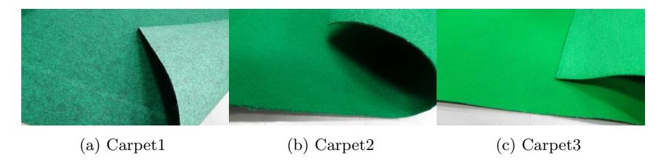
In order to evaluate the effectiveness of the proposed dribbler, we measured the ball-holding time when the robot rotates with a ball. We used three types of carpets in experiment. These pictures are shown in Fig.4. The The material of all carpets is 100% polypropylene. Carpet1 shown in Fig.4(a) is used in our playing-field. The surfaces of (a) Carpet1 and (b) Carpet2 shown in Fig.4 are similar, and they are relatively smooth and their friction is small. On the other hand, the surface of (c) Carpet3 is rough and hard, and its friction is larger.
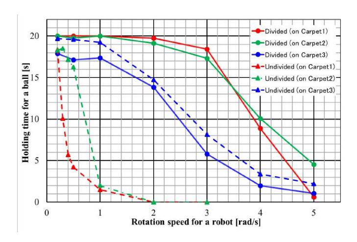
Figure 5 shows experimental results. The horizontal axis shows the rotation speed of a robot, and the vertical axis shows the average holding-time. It was shown as 20 seconds in case of keeping 20 more over seconds. Three values were used as the rotation speed of dribbling-motor in the range of about 75 s*−*1 to 105 s −1 (4500rpm to 6300rpm). The data plotted in Fig. 5 show the their average.
From the results in Fig. 5, when the robot's rotation speed exceeds 1 rad/s, it shows that the previous undivided-dribbler can hardly hold a ball. On the other hand, in present divided-dribbler, it is found that the robot can hold a ball for 15 over seconds under the rotation speed of 3 rad/s (about 180 deg/s) without changing the shape of the dribbling-bar or the dribbler unit.
It was also found, however, that the effect of divided-dribbler is relatively ineffective in case of the material with a high friction coefficient to a ball, such as (c) Carpet 3 shown in Fig.4. This is due to the fact that a ball rotates at a low speed because our system cannot work the feedback corresponding to the magnitude of the friction. In most of general playing-field, nevertheless, it is considered effective if the robot can hold about 15 seconds rotating at 3 rad/s. Therefore, it can be said that this experiment shows the effectiveness of divided-dribbler.
3 Electrical system
We have used 2.4GHz band XBee-PRO as a wireless communication module. But, as increasing of the field size and the number of the robots, the many troubles attributed to low-power wireless modules have occurred. Thus, in order to improve the accuracy of pass-play and obstacle avoidance, we decided to use the sensors. In addition, Vision-Blackout problem are also tried to solve. In our previous circuit boards, it was difficult to add the sensors easily and to change to the other devices. Furthermore, it cannot also perform the bidirectional communication, so we developed a new circuit board to clear up their problem. In this section, we describe the outline of the new circuit board, and about the handling to Vision-Blackout problem by use of the local camera.
3.1 Electrical main board
Up to now, we have had some problems for communication and motor control in robots.
The former was attributed to the use of XBee or XBee-PRO as a wireless communication module. This device is based on the IEEE 802.15.4 standard, and has the advantages of low cost, low power drive, and easy handling because it can simply communicate with the microcomputer using the UART method. However, the output power of XBee series are limited with up to 10 mW by the Radio Law of Japan, and communication interruption has come to occur frequently due to the interference with the radio wave of 2.4 GHz band Wi-Fi device.
The latter was attributed to the fact that it was only used the rotation speed of the motor as feed back control. The wheel is connecting directly Maxon's 70 W brushless DC motor without reduction gears, but the motor is only controlled by an encorder and is no current feedback. As the result, it was not able to detect the slipping and to run smoothly. In an actual match, our AI system makes a correction based on SSL-Vision for the robot's motion, but if the distance to a target is short, it will vibrate. Especially, it is difficult to control on direct-drive compared with gear-drive, when the motor speed is low.
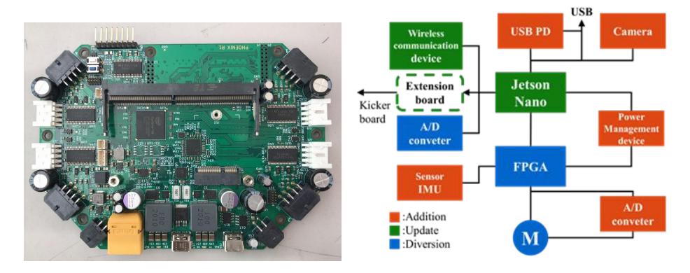
Therefore, in order to clear up above problems, we designed and developed a new circuit. For designing a new circuit board, we referred to the paper of other teams, for example, TIGERs Mannheim[2] and ZJUNlict[3]. Figure 6 and 7 show the new board and its configuration, respectively.
First, we changed the MCU from a 32-bit microcomputer to Jetson Nano[4] made by NVIDIA. This makes it possible to use Wi-Fi card generally mounted on computers, making it easy to use device that comply with domestic Radio Law. The Wi-Fi card used in the new circuit board are 8260NGW and 8265NGW made by Intel. These Wi-Fi cards can use the Wi-Fi 5.0 GHz band, which we believe allows us to use a less congested band. In RoboCup Asia-Pacific 2021 Aichi Japan held in 2021, we evaluated the communication performance of new robot, and confirmed no major communication trouble.
In Jetson Nano on main board, we need to do the operation of boot or shutdown. Therefore, we used GreenPAK[5], a power management device to manage the applied voltage to the board. That is, the power supplied for driving motors and for controls can be made a common, or the voltage can be also applied only to Jetson Nano without applying the voltage to motor-control system.
USB Power Delivery (USB PD) can also use to supply the power to main circuit board. When the power is supplied from USB PD, GreenPAK controls motor-control system not to supply the voltage. While USB PD is supplying voltage, a Lipo-battery can be replaced without shutting down operation of Jetson Nano. Development using GreenPAK is not difficult because it can be developed using GUI. Another big advantage of use of Jetson Nano is possible to use a local camera. This is described in detail section 3.2.
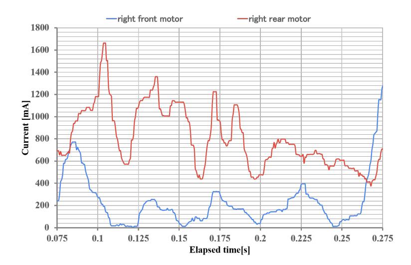
Due to the high manufacturing cost of the main circuit, it is not easy to change. Therefore, the functions envisaged change, such as ball sensors and communication tool on Kicker board, were consolidated in the extension board. For the electronic devices related to the motor control, a shunt resistor of 3 mΩ and ICM-42688[6] which is an IMU made by TDK, were added. By adding a shunt resistor, it is possible to measure the applied current to the motor. The applied current is input to motor-control system through the CIC filter and the Median filter. Figure 8 shows the time-series waveform of measured current when the robot moved to the right-direction. The horizontal axis shows the elapsed time after robot moves to right-direction and the vertical axis shows the measured current. In Fig.8, the current in time-range from 0.1s to 0.25s on the right-front motor shows a lower value than that of other time-range, it suggests occurrence of slipping. Therefore, by using this current information, the improvement of attitude control of motor can be expected.
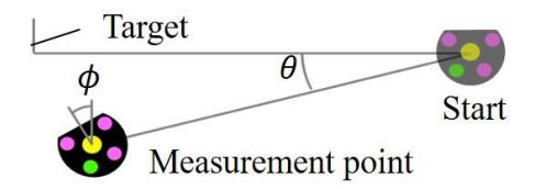
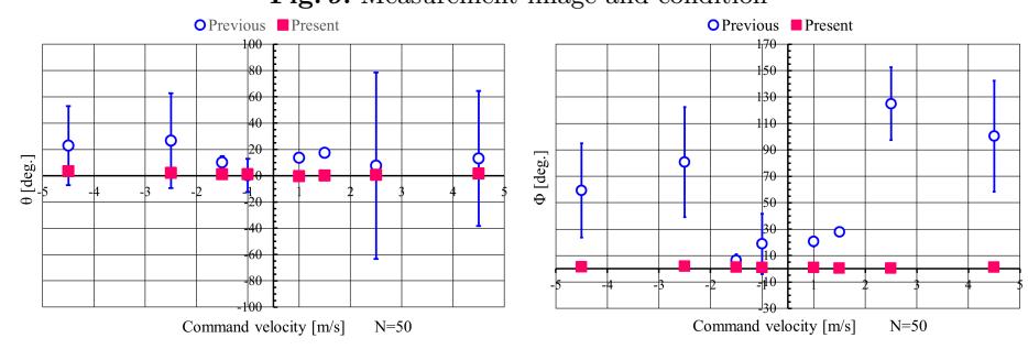
Acceleration data and gyro data could be also obtained with the introduction of the IMU (ICM-42688). Using this information as feedback data, we conducted an experiment to run the robot without correction from AI. Thus, when the robot run straight sideways from the Start point to the Target point, the correction performance using only the IMU data was evaluated using the angle symbol shown in Fig.9. Figures 10 and 11 show the results. The dots and bars indicate the mean value and deviation of errors for θ or φ, respectively. The horizontal axis shows the elapsed time after robot moves. The enlarged view drawn lower indicates smaller error and good performance for the new circuit board.
The spatial layout of omni-wheel in our robots is asymmetrical in the direction of front-back and left-right because the dribble mechanism is widely installed in front of the robot. Therefore, a robot slips easily on the left-right direction and results unfortunately rotation of the robot itself. But in Fig,10 and 11, we can see clearly that the running performance of the robot using new board equipped with IMU will be more stable than that of the previous robot. This is mainly due to the feedback provided by the gyro data. Previous robots could only use the rotation speed of a motor as feedback data, but the new robot can use gyro and acceleration data, which will enable us smarter attitude control. As mentioned above, we confirmed improvement for the performance of new circuit board.
3.2 Dealing with the vision blackout and communication delay by use of a local camera
The current system has the following problems.
- Because of the Vision-Blackout, the position of a ball cannot be specified.
- Disconnection or delay in wireless communication.
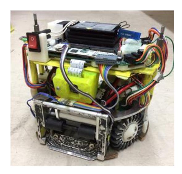
To solve this problem, we tried to add a local camera on the robot. As shown in Fig.12, the Raspberry Pi camera module was mounted on front of the robot at a height of 8.5 cm and a horizontal downward angle of 12.5 °. The robot can recognize a ball with a local camera within a range of 2 meter ahead and viewing angle of about 40 °. Hardware configuration is already shown in Fig.7 (p.5). The data from the local camera is processed by Jetson Nano. After that, it is used for the motor control by FPGA.
Figure 13 shows the confirmation process of the ball tracking-performance of the robot using only a local camera. Open CV is used to receive the local vision image and to configure the structure of the image data. K^P is the proportional constant used for the position control of the robot. In the filter process, first, the evaluation values {Er, Eg, Eb} of each RGB are calculated from the RGB values {Vr, Vg, Vb} of the pixel using eq.(1)-(3). Next, each evaluation value is weighted. Then, the average value Eall for the entire pixel using eq.(4) is obtained. Eq.(4) is used to determined a ball (or other) based on whether the value exceeds a appropriate threshold value indicated in eq.(5). The calculation parameters and constants used in the equations were determined through actual experimental environment. Finally, the speed control is done by FPGA. Please see the video for qualification in 2022.
$$E_r = V_r \tag{1}$$
$$E_g = \min(4V_g, 255, 2(255 - V_g)) \tag{2}$$
$$E_b = -V_b \tag{3}$$
$$E_{all} = \frac{7E_r + 10E_g + 5E_b}{7 + 10 + 5} \tag{4}$$
$$E_{all} > 205 \tag{5}$$
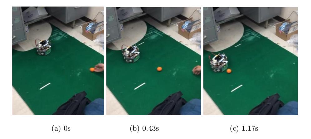
Using above system, we set a robot on the playing-field and moved a ball to front of the robot as shown in Fig. 14. As the result, we confirmed that the robot can correctly recognize a moving ball and calculate the coordinates. In present, by comparing the difference between the local vision and global vision for the position-coordinates of ball and robot, it is confirmed that it can be used to correct the command value of AI.

4 Software system
(section placeholder for subsections)
4.1 Decision-Making Algorithm using Monte Carlo Tree Search
In decision making of robot systems, realization of cooperative behavior by multiple robots, variability of constraints, and explainability are considered to be important issues. We proposed a decision-making algorithm that combines Monte Carlo Tree Search (MCTS) and neural network as a method to solve these problems, and have implemented it in our software [1]. In order to improve the performance of this algorithm, we have improved the accuracy of the neural network and increased the speed by parallelization.
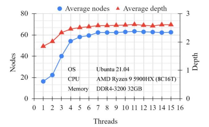
Parallelization of MCTS In order to use CPU efficiently, we have introduced Tree parallelization[7], in which multiple threads share a single game tree. In Tree parallelization, exclusion control leads to a decrease in search efficiency. Figure 15 shows the results for testing the effect of parallelization on 100 different situations. The horizontal axis shows the number of threads, and the vertical axis shows the average number of nodes generated and the average depth. In the environment used for this verification, it was found that parallelization was effective up to about 7 threads.
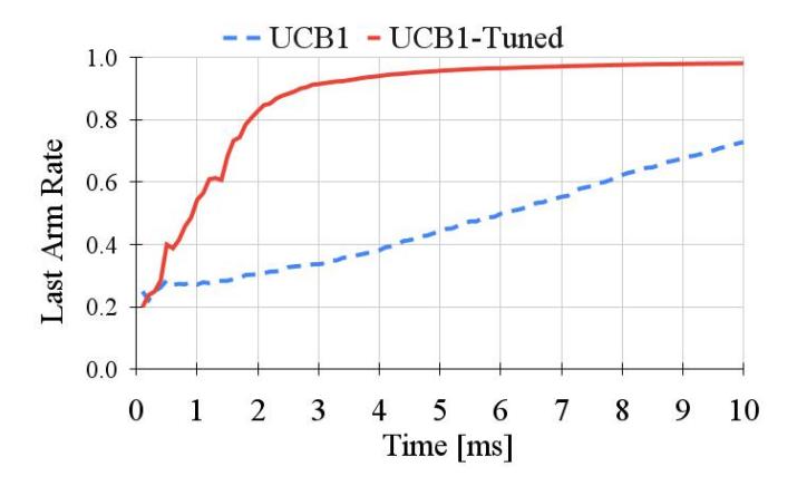
Validation of the algorithm used for the Selection We have been using UCB1 as an algorithm for node selection in MCTS. In this study, we implemented UCB1-Tuned [8] (eq. (6)), which is derived from UCB1, and evaluated their performance.
$$\underset{i=1...k}{\operatorname{arg,max}} \left( \hat{\mu_i} + \sqrt{\frac{\ln \sum_j n_j}{n_i} \min \left( \frac{1}{4}, \hat{\sigma_i}^2 + \sqrt{\frac{2 \ln \sum_j n_j}{n_i}} \right)} \right) \tag{6}$$
Where ˆμ^i is the expected value of the reward of legal move i, n^i is the number of visits of legal move i, and ˆσ^i 2 is the variance of the reward of legal move i. Figure 16 shows the selection rate of the last arm as a percentage of all choices for UCB1 and UCB1-Tuned in a given phase. The horizontal axis shows the time and the vertical axis shows the percentage of the last arm among all selections at that time. Here, the last arm is assumed to be the node with the highest number of visits at 10 ms (which is the same move for both algorithms). UCB1-Tuned converges the selection in a shorter time. It means that it can search more efficiently than UCB1.
Improving the inference performance of Neural Networks Our previous neural network for transitivity inference between nodes had an accuracy of 84%. In this study, we reviewed the structure of the network and the training data to improve the inference performance. In the new network, we replaced the Swish function with the ReLU function to reduce the computational complexity. For training the network, we used 2000 pieces of data (compared to 150 pieces in the past). Table 1 shows the results of the performance evaluation. The accuracy of the new network is 94%, which is an improvement in inference performance over the previous network.
Probability predicted by Neural Network on Confusion Matrix (100 samples)
| Data \ Predicted probability | <0.5 | ≥0.5 | Recall |
|---|---|---|---|
| Failure | 47 | 3 | 0.94 |
| Success | 3 | 47 | 0.94 |
| Precision | 0.94 | 0.94 | |
| Accuracy | 0.94 |
4.2 Angular correction to improve kicking performance
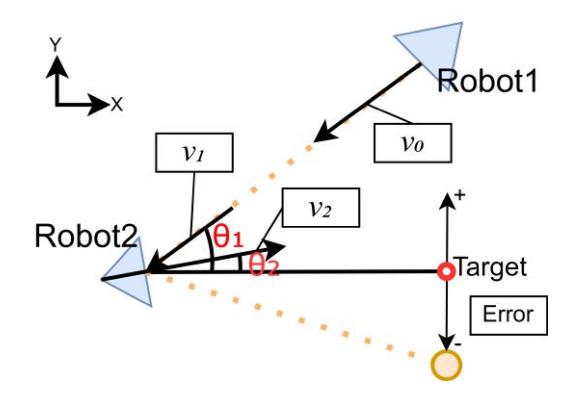
Currently, in our software, in a scene where a robot passes or shoots a ball, it often receives a moving ball once, then turns, and then kicks. That is, direct-shooting with single touch is rarely performed. This is because the angle correction has not been performed on direct-shooting. Especially, in case of the shooting from a wide angle, the trajectory of a ball deviates substantially from the target position if angle correction is not taken into account. This deviation is attributed to the momentum of a ball before and after kicking. In order to improve scoring performance, it important to increase the success rate in situation where the direct-shooting is possible. In this section, we consider about the angle correction for direct-kicking. The configuration and the parameters used in experiment are shown in Fig.17 and Table 2, respectively.
$$Error = B - A(v_1 sin\theta_1 - v_2 sin\theta_2) \tag{7}$$
$$\theta_2 = Sin^{-1} \left( \frac{v_1}{v_2} sin\theta_1 - \frac{B}{Av_2} \right) \tag{8}$$
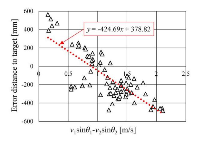
Figure 18 shows the relationship between the difference (v1sinθ1-v2sinθ2) in the y-direction component of the ball velocities before and after kicking and the error distance to the target. The dotted line shown in Fig.18 represents an linear approximation of the plotted data. Using the slope A and intercept B of this linear line, the equation is shown by eq.(7). By substituting zero for the left side of eq.(7), arbitrary parameter that makes the error zero can be derived. Therefore, the correction angle θ^2 to Target position is expressed by eq.(8) from eq.(7).
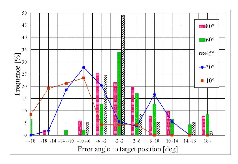
Obtained correction function for θ^2 was introduced into AI system and its performance was evaluated. The result is shown in Fig.19. According to the results in Fig.19, the correction effect for θ^2 is insufficient in case of the narrow angles less than 30 ° to receive the ball. On the other hand, it is shown the effectiveness in that of wide-range angles wider than 45 °. This might be attributed to the accuracy of the analyzed correction function. In the actual game, we need to consider using the correction function depending on the situation of the field. For example, the correction function should not be used for narrow angles, but only for wide angles.
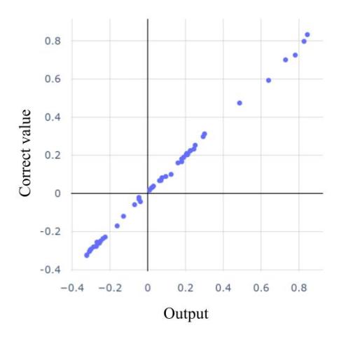
Figure 20 shows the comparison between the correct value and the output value which obtained from constructed neural network using the experimental data shown in Fig.18 as training data. In this result, it can be seen that the output from neural network show good agreement with correct value. Based on the result, we will try to introduce the angle correction system. It is not easy to derive an effective correction function under all conditions, but we think it is possible to confirm the effectiveness by practice during the setup-period of the competition.
Parameter used in the experiment for angular correction
| symbol | comment |
|---|---|
| v1 | Ball speed given by Robot1 |
| v2 | Ball speed given by Robot2 |
| θ1 | Angle between Robot1 and Target relative to Robot2 |
| θ2 | Tilt angle (correction angle) of Robot2 to Target position |
Acknowledgments
This work was supported in part by JSPS KAKENHI Grant Number 20K03263, Grant-in-Aid from the Chuden Foundation for Education and The Nitto Foundation in Japan, respectively.
References
- Yusei Naito, Shin Ohno, Yuta Imaeda, Akihito Odanaka, Yasutaka Tsuruta, Ryoma Mitsuoka, Taisuke Tane, Masato Watanabe and Toko Sugiura, KIKS Extended Team Description for RoboCup 2020; https://ssl.robocup.org/wp-content/uploads/2020/03/2020_ETDP_KIKS.pdf (2020.03)
- TIGERs MANNHEIM, TIGERs MANNHEIM publications; https://www.tigers-mannheim.de/index.php?id=65
- ZJUNlict, ZJUNlict github Main Board; https://github.com/ZJUNlict/Main_Board
- NVIDIA, Jetson Nano; https://www.nvidia.com/en-us/autonomous-machines/embedded-systems/jetson-nano
- Dialog Semiconductor, GreenPAK; https://www.dialog-semiconductor.com/products/greenpak
- TDK, ICM-42688-P; https://product.tdk.com/system/files/dam/doc/product/sensor/mortion-inertial/imu/data_sheet/ds-000347-icm-42688-p-v1.2.pdf
- Guillaume M.J-B. Chaslot, Mark H.M. Winands, and H. Jaap van den Herik: Parallel Monte-Carlo Tree Search, Comp. Games, 6th Inter. Conf; https://dke.maastrichtuniversity.nl/m.winands/documents/multithreadedMCTS2.pdf (2008).
- Peter Auer, Nicolò Cesa-Bianchi, Paul Fischer: Finite-time Analysis of the Multiarmed Bandit Problem, Machine Learning 47, 235-256; https://link.springer.com/article/10.1023/a:1013689704352 (2002)