RoboDragons 2022 Extended Team Description

Masahide Ito, Yuta Ando

School of Information Science and Technology, Aichi Prefectural University 1522-3 Ibaragabasama, Nagakute, Aichi 480-1198, JAPAN

https://robodragons.github.io/

Abstract RoboDragons is a team of the RoboCup Soccer Small Size League (SSL) from Aichi Prefectural University, Japan. In RoboCup 2022, they will use the seventh-generation robots—developed in 2016 for the SSL competition. This paper shares the technical information of system updates implemented between 2020 and 2022. In particular, focusing on the upper-layer control system, a trajectory tracking controller in consideration of obstacle avoidance is presented.

Introduction

RoboDragons is a team of Aichi Prefectural University (APU) participating in the Small Size League (SSL) of RoboCup Soccer. This team originated from Owaribito—a joint team between APU and Chubu University—which was founded in 1997. In 2002, since two universities have been ready to manage each individual team, APU built a new team, RoboDragons. After that, RoboDragons has been participating in the SSL for more than 18 years, including activities as CMRoboDragons—a joint team with Carnegie Mellon University in 2004 and 2005. Our best record was the second place in 2009. We also finished twice in the third place (2007 and 2014) and four times in the fourth place (2004, 2005, 2013, and 2016). In RoboCup 2021, we placed seven out of 16 teams in Virtual Tournament and also nine out of 12 teams in Hardware Challenge.

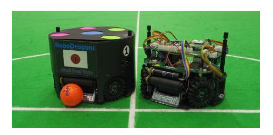
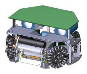
Similarly to last five years, the seventh-generation (7G) robots (Fig. 1) will be used in RoboCup 2022. This generation has developed in 2016 and the first competition was RoboCup 2017. See our ETDP 2017 [1] for the specification of the hardware and software of the 7G robot. RoboCup 2017 was the first time for the 7G robots to compete the official SSL games with the other teams. After that, based on the issues found in some official/friendly matches and daily development, we have tried to improve the hardware and software. From 2017 to 2018, to widen the ball-touchable area of the dribbling roller, some spaces on the side brackets of the dribbler were whittled down; to improve motion control of the robots, a trajectory tracking controller based on linear model predictive control was developed [2]. From 2018 to 2019, the small wheels of the omniwheels were replaced for their more smooth mobility and less maintenance; to increase the successful rate of ball placement starting near the wall even if the dribbler does not work for keeping the ball, a skill to kick a ball to the wall diagonally was added [3]. From 2019 to 2020, to improve the dribbler so as to keep the ball more, different kinds of rollers were evaluated; a local vision system and control algorithm for SSL-Vision Blackout Challenge were developed [4].

This paper provides the technical information of system updates that RoboDragons have implemented between 2020 and 2022. In particular, focusing on the upper-layer control system, an upper-layer controller is improved so as to realize not only trajectory tracking but also obstacle avoidance. Obstacle avoidance indicates that the robot moves between the initial and target positions so as not to collide an obstacle on the way.

Trajectory Tracking Controller in Consideration of Obstacle Avoidance

Two-layered Control System

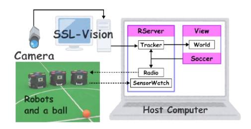
Robotic soccer in the SSL is characterized as fast-paced games with real robots. This feature is mainly provided by a combination of a global vision system called as SSL-Vision, wireless network, omni-directional mobile robots, and a centralized system as depicted in Fig. 2. What effectively combines those stuff and maximize the performance is a motion controller in each team software.

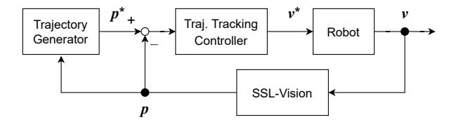
As shown in Fig. 3, RoboDragons adopts a two-layered control system that consists of the upper and lower layers [1]. The upper-layer control system (Fig. 3 (a)) is for trajectory tracking control of the robot; the lower-layer one (Fig. 3 (b)) is for angular velocity control of wheel motors. What we want to control as we desire are robot players while what drives each robot are wheel motors. Normally, the sampling and control rates of the lower-layer control system are faster than the upper-layer one. In this meaning, the upper- and lower-layer control systems are also called as outer- and inner-loops, respectively.

The upper-layer control system (Fig. 3 (a)) is always sampling the raw data of the robots' and ball's positions provided from SSL-Vision. Although omitted in Fig. 3 for simplicity, the following process of three steps conducts between SSL-Vision and Trajectory Generator:

• Step 1: By filtering the SSL-Vision raw data with an extended Kalman filter, the team Artificial Intelligence (AI) properly recognize a situation on the field and then chooses an appropriate strategy;
• Step 2: To try to achieve the chosen strategy, the corresponding roles are assigned to the robots; and
• Step 3: A target position is given for each robot. The target position is modified by using Rapidly-exploring Random Tree (RRT) if there is any obstacle on a path between the current and target positions.

In the Trajectory Generator block, a velocity trajectory for reaching the target position at a desired time is generated as a first-order polynomial. By integrating it, the corresponding position trajectory is obtained. In the Trajectory Tracking Controller block, a control law so as to compensates the error between planned and actual trajectories runs. At the end, the controller outputs the velocity command and then sends it via wireless communication to the robots.

On the other hand, the lower-layer control system (Fig. 3 (b)) is running onboard based on the velocity command provided from the upper-layer controller. The velocity command with respect to the robot itself is transformed into the one with respect to the wheels through the inverse kinematics derived from the mechanical structure. At each wheel, the actual angular velocity is followed to the command via a PID controller. Finally, the robot realizes a behavior following the command.

As presented in [2], RoboDragons have introduced a trajectory tracking controller based on Model Predictive Control (MPC) [5]. Since 2018, the mathematical model used for state prediction in the controller has been extended as in [8] and also obstacle avoidance has been considered as one of constraint conditions in [9]. This ETDP will share a basic manner to design a linear MPC-based trajectory tracking controller in consideration of obstacle avoidance.

MPC-based Trajectory Tracking Controller in Consideration of Obstacle Avoidance

MPC is a control scheme to online solve a control optimization problem under system constraints. In particular, the main feature of MPC is that control optimization exploits future system behavior (state) predicted by its mathematical model. The demerit of MPC is to cost high for its computation. In meantime, it is important for real-time property of control-loop to control real robots. For saving computational cost, similarly to in [2], let a controller design be limited into the linear MPC framework. Then, a control objective as a cost function must be formulated in the quadratic form with linear inequality constraints. In this framework, CVXGEN [6, 7] is useful because it generates a C code to fast solve a linear MPC problem. This subsection presents how to handle obstacle avoidance as a linear inequality constraint in a linear MPC problem.

A basic recipe to develop a linear MPC controller using CVXGEN is as follows:

• Step 1: Derive a linear state-space model (a pair of state and output equations) of the controlled object as a mathematical model;
• Step 2: Formulate a control objective and system constraints as a constrained optimization problem;
• Step 3: Code the constrained optimization problem using the CVXGEN format in the website [7];
• Step 4: Generate the corresponding C code at the website and download it;
• Step 5: Merge the generated code with the other code of the team AI.

As for the first three steps, the detail of each step is described in the following paragraphs.

Step 1. A continuous-time state-space model of the SSL robot can be represented as

$$\frac{\mathrm{d}}{\mathrm{d}t}\boldsymbol{x}(t) = \begin{bmatrix} \alpha_x & 0 & 0\ 0 & \alpha_y & 0\ 0 & 0 & \alpha_\omega \end{bmatrix} \boldsymbol{u}(t - t_w),\tag{1a}$$

$$\mathbf{y}(t) = \mathbf{x}(t),\tag{1b}$$

where $\boldsymbol{x}$ is a state vector consisted of the robot's position and orientation, $\boldsymbol{u}$ is a control input vector consisted of the velocity commands to the robot, $\boldsymbol{y}$ is an output—measurable state—vector, $\alpha_x$, $\alpha_y$, and $\alpha_\omega$ are scaling factors between the actual and command velocities, and $t_w$ is dead-time, respectively. What a linear MPC controller exploits for state prediction is a discrete-time state-space model. By discretizing Eqn. (1) by a sampling time $T_s$, the following discrete-time representation is obtained:

$$\boldsymbol{x}(k+1) = \boldsymbol{x}(k) + T_s \begin{bmatrix} \alpha_x & 0 & 0 \ 0 & \alpha_y & 0 \ 0 & 0 & \alpha_\omega \end{bmatrix} \boldsymbol{u}(k-H_w), \tag{2a}$$

$$\mathbf{y}(k) = \mathbf{x}(k),\tag{2b}$$

where $t = kT_s$ and $H_w := \lfloor t_w/T_s \rfloor$, respectively.

Step 2 (the former part). One of typical control objectives is to drive the robot into the target position/trajectory. This can be written as the following cost function:

$$V(k) = \sum_{i=H_w}^{H_p} |\hat{\boldsymbol{y}}(k+i|k) - \boldsymbol{y}^(k+i|k)|{\boldsymbol{Q}(i)}^2 + \sum{i=0}^{H_u-1} |\hat{\boldsymbol{u}}(k+i|k) - \boldsymbol{u}^(k+i|k)|_{\boldsymbol{\mathcal{R}(i)}}^2, \quad (3)$$

where $\hat{\boldsymbol{u}}$ and $\hat{\boldsymbol{y}}$ are predicted input and output in the MPC controller, $\boldsymbol{y}^{\star}$ and $\boldsymbol{u}^{\star}$ are set-point trajectories (can be set to set-points or reference trajectories) for $\hat{\boldsymbol{u}}$ and $\hat{\boldsymbol{y}}$, $\boldsymbol{\mathcal{Q}}$ and $\boldsymbol{\mathcal{R}}$ are weighting matrices, and $H_p$ and $H_u$ ($\leq H_p$) are prediction horizon for $\hat{\boldsymbol{u}}$ and $\hat{\boldsymbol{y}}$, respectively. Note that $\boldsymbol{y}^{\star}(k+i|k)$ and $\boldsymbol{u}^{\star}(k+i|k)$ are replaced with $\boldsymbol{y}^{\star}=$ const. and $\boldsymbol{u}^{\star}=\boldsymbol{0}$, respectively, when considering a set-point regulation problem instead of a trajectory tracking problem.

Step 2 (the latter part). Subsequently, consider system constraints. Due to actuator saturation, control inputs and their rates are normally constrained such as

$$|u_j(k)| < \bar{v}_j, \tag{4}$$

$$|u_j(k) - u_j(k-1)| \le \bar{a}_j T_s,\tag{5}$$

where $\bar{v}_j$ and $\bar{a}_j$ are soft limiters of the corresponding velocity and acceleration $(j=1,2,3,,k=0,1,\cdots,H_u-1)$, respectively. In addition to this, this paper handles obstacle avoidance as one of state constraints. Suppose that any obstacle is static and also is shaped as a circle. Considering a obstacle itself as a prohibited area, which is formulated by the following inequality in the quadratic constraint format:

$$|^{w}\boldsymbol{p}(k) - {}^{w}\boldsymbol{p}{o}|{2} \ge r_{o},\tag{6}$$

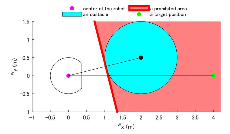
where $^{w}\boldsymbol{p}$, $^{w}\boldsymbol{p}{o}$, and $r^{o}$ represents the robot position, the position and radius of the obstacle, respectively. A quadratic constraint as in Eqn. (6) cannot be handled in a linear MPC manner, it can be approximated to the linear one. By linearly approximating Eqn. (6) based on Taylor series expansion at a tangent point $^{w}\boldsymbol{p}(k) = {}^{w}\boldsymbol{p}{c}$, the following inequality

$$({}^{w}\boldsymbol{p}{c} - {}^{w}\boldsymbol{p}{o})^{\mathsf{T}} {}^{w}\boldsymbol{p}(k) > {}^{w}\boldsymbol{p}{c}^{\mathsf{T}} ({}^{w}\boldsymbol{p}{c} - {}^{w}\boldsymbol{p}_{o}), \tag{7}$$

where $^{w}\boldsymbol{p}^{c}$ is a vector indicating a point that is intersection of the circumference of the obstacle circle and the segment between the robot and obstacle. See Fig. 4 for a prohibited area given by Eqn. (7).

Step 3. On the CVXGEN website [7], translate the constrained optimization problem into a CVXGEN code. A sample code is shown in Source Code 1.1.

Source Code 1.1: description.cvxgen

1 dimensions
2 n = 3 # of state
3 m = 3 # of input
4 l = 3 # of output
5 Hp = 10 # prediction horizon
6 Hu = 5 # control horizon
7 Hw = 1 # dead - time ( time delay )
8 end
10 parameters
11 A(n ,n ) # system matrix
12 B(n ,m ) # input matrix
13 C(l ,n ) # output matrix
14 Q(l ,l ) psd # for state cost
15 R(m ,m ) psd # for input cost
16 x[Hw -1] (n) # initial state
17 v1bar [ k] nonnegative , k =0.. Hu -1
18 v2bar [ k] nonnegative , k =0.. Hu -1
19 a1bar [ k] nonnegative , k =0.. Hu -1
20 a2bar [ k] nonnegative , k =0.. Hu -1
21 u_p (m)
22 Poscoef [k] (1 , n) , k= Hw .. Hp
23 r_limit [k], k= Hw .. Hp
24 y_cmd ( l)
25 end
26
27 variables
28 x[k ]( n) , k= Hw .. Hp
29 u[k ]( m) , k =0.. Hu -1
30 y[k ]( l) , k= Hw .. Hp
31 end
33 minimize
34 sum [k= Hw .. Hp ]( quad ( y[k] - y_cmd ,Q )) + sum [k =0.. Hu -1]( quad (u[k ],R) )
35 subject to
36 x[k] == A* x[k -1] + B *u[k -1] , k= Hw .. Hu
37 x[k] == A* x[k -1] + B *u[Hu -1] , k = Hu +1.. Hp
38 y[k] == C* x[k] , k = Hw .. Hp
40 abs (u[k ][1]) <= v1bar [k], k =0.. Hu -1
41 abs (u[k ][2]) <= v2bar [k], k =0.. Hu -1
42 abs (u [0][1] - u_p [1]) <= a1bar [0]
43 abs (u[k ][1] - u[k -1][1]) <= a1bar [ k], k =1.. Hu -1
44 abs (u [0][2] - u_p [2]) <= a2bar [0]
45 abs (u[k ][2] - u[k -1][2]) <= a2bar [ k], k =1.. Hu -1
47 Poscoef [k ]* x[k] <= r_limit1 [k ], k= Hw .. Hp
48 end

Experimental verification

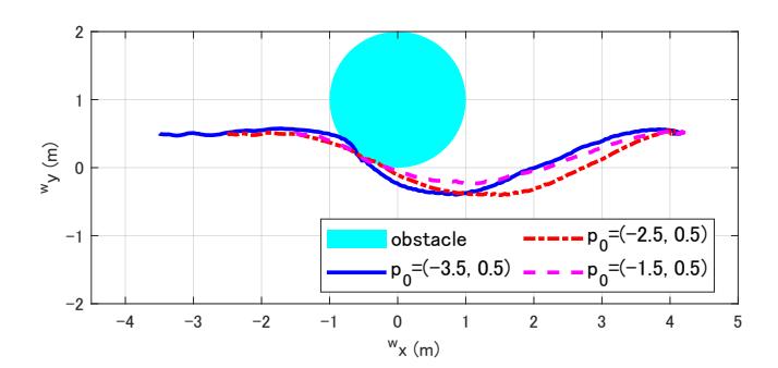
The effectiveness of the designed controller is evaluated via some experiments with a real robot. The experiments were performed as the following setting:

• The initial position of the robot, p0, were chosen out of the three kinds of ones: (−3.5 m, 0.5 m), (−2.5 m, 0.5 m), and (−1.5 m, 0.5 m);
• The target position p⋆ was set to (−3.5 m, 0.5 m); and
• There is a virtual obstacle of between the initial and target positions of the robot. The obstacle describes a circle with the radius of 1 m (i.e., r^o = 1 m), whose center is placed at (0 m, 1 m).

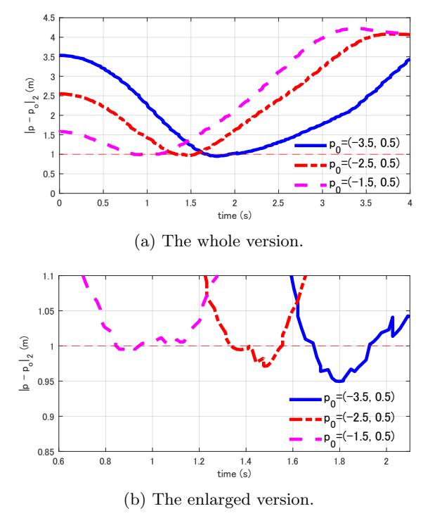
Figures 5 and 6 visualize the experimental results performed with the following parameters: α = diag{0.9822, 0.9786, 0.9528}, T^s = 1/60 s, H^p = 10, H^u = 5, H^w = 1, Q = diag{500, 100, 100}, and R = diag{15, 15, 15}, respectively. Fig. 5 presents the trajectories that the robot actually moved on the field; Fig. 6 shows the time responses of a distance between the robot and obstacle. If the plotted data in this figure lies on and below the red broken line, the meaning is that the robot invades the obstacle.

From Figures 5 and 6, it can be observed that the robot was primarily avoiding the obstacle but slightly invading the obstacle area [3]. This result, however, is not bad because the SSL rules restricts the radius of an SSL robot to be less than 0.09 m. It implies that the radius of a virtual circular wall just has to be appropriately longer than the one of the real obstacle. Also, it can be seen that how much the robot invades the obstacle depends on the initial position. The reason is that the control problem considered here is set-point regulation and also the initial position, i.e., distance between the initial and target positions, affects the acceleration of the robot near the obstacle.

Concluding Remarks

This paper has shared the technical information of RoboDragons 2022. The main description is to design and validate an MPC-based trajectory tracking controller in consideration of avoiding obstacles.

Acknowledgement

The authors would like to thank the other active RoboDragons 2022 members, Nakayama, M., Ban, K, Kakeno, N., Kashiwamori, F., Suzuki, N., Yamada, M., Fujita, F., Shibata, M., Sugiura, K., Suzuki, T., Kato, S., Agatsuma, S., Shimizu, T., Honobu, K., Miyazaki, Y., and Mori, K. This work was partially supported by The Nitto Foundation and Aichi Prefecture.

References

1. Adachi, Y., Kusakabe, H., Suzuki, R., Du, J., Ito, M., and Naruse, T.: "Robo-Dragons 2017 extended team description," RoboCup Soccer Small Size League, 2017. Available online: https://ssl.robocup.org/wp-content/uploads/2019/01/2017_ETDP_RoboDragons.pdf (accessed on 1 Feb 2022).
2. Ito, M., Kusakabe, H., Adachi, Y., Suzuki, R., Du, J., Ando, Y., Izawa, Y., Isokawa, S., Kato, T., and Naruse, T.: "RoboDragons 2018 extended team description," RoboCup Soccer Small Size League, 2018. Available online: https://ssl.robocup.org/wp-content/uploads/2019/01/2018_ETDP_RoboDragons.pdf (accessed on 1 Feb 2022).
3. Ito, M., Suzuki, R., Isokawa, S., Du, J., Suzuki, R., Nakayama, M., Ando, Y., Umeda, Y., Ono, Y., Kashiwamori, F., Kishi, F., Ban, K., Yamada, T., Adachi, Y., and Naruse, T.: "RoboDragons 2019 extended team Description," RoboCup Soccer Small Size League, 2019. Available online: https://ssl.robocup.org/wp-content/uploads/2019/03/2019_ETDP_RoboDragons.pdf (accessed on 1 Feb 2022).
4. Ito, M., Nakayama, M., Ando, Y., Adachi, Y., Du, J., Suzuki, R., Ono, Y., Kashiwamori, F., Ban, K., Isokawa, S., Yamada, T., and Naruse, T.: "RoboDragons 2020 extended team Description," RoboCup Soccer Small Size League, 2020. Available online: https://ssl.robocup.org/wp-content/uploads/2020/03/2020_ETDP_RoboDragons.pdf (accessed on 1 Feb 2022).
5. Maciejowski, J.M.: "Predictive Control with Constraints," Prentice Hall, 2000.
6. Mattingley, J. and Boyd, S.: "CVXGEN: A code generator for embedded convex optimization," Optimization and Engineering, Vol. 13, No. 1, pp. 1—27, 2012. doi: 10.1007/s11081-011-9176-9.
7. GVXGEN: Code Generation for Convex Optimization. Available online: https://cvxgen.com/docs/index.html (accessed on 1 Feb 2022).
8. Suzuki, R. and Ito, M.: "Trajectory tracking controller based on linear model predictive control for omni-wheeled mobile robots with velocity command limits," Proceedings of the fifth IEEJ International Workshop on Sensing, Actuation, Motion Control, and OptimizatioN (SAMCON'19), Paper No. V1-7, Chiba, Japan, March 2019.
9. Ando, Y. and Ito, M.: "Obstacle avoidance of omnidirectional mobile robots in consideration of motion performance," Proceedings of the seventh IEEJ International Workshop on Sensing, Actuation, Motion Control, and OptimizatioN (SAMCON'21), pp. 394–395, Chiba, Japan, March 2021.