RoboIME: On the road to RoboCup 2022
Felipe W. V. da Silva, Antˆonio S. G. Pereira, Vinicius de F. L. Moraes, Gabriel H. M. Silva, Mayara R. Mendon¸ca, Gabriel M. Lima, Jos´e L. de O. Schramm, Henrique Barreto, Iasmin C. Mathias, Lucio E. Horie, Enzo G. Frese, Pedro V. Rocha, Renato da P. Alves, Marcus V. P. dos Santos, Marcos C. Antunes, L´eo V. C. Vasconcelos, Isabel C. de Freitas, Lucas G. Corrˆea, Gabriel B. da Concei¸c˜ao, Carla S. Cosenza, Lucas B. Germano, Matheus Bozza, Luis D. P. de Farias, Jo˜ao G. O. C. de Melo, Nicolas S. M. M. de Oliveira, Gustavo C. K. Couto, Herbert Azevedo, Luiz R. L. Rodrigues, Paulo F. F. Rosa
Instituto Militar de Engenharia, Rio de Janeiro, Brasil
Abstract This paper describes the electronic, mechanical, and software designs developed by the RoboIME Team to join the RoboCup 2022. The overall concepts are in agreement with the rules of Small Size League 2022. This is the ninth time RoboIME participates in the RoboCup tournament.
1 Introduction
RoboIME is a Small-Size League team from the Instituto Militar de Engenharia, IME - Brazil, and this is the 17th time the team participates in a competition. The team has already gotten good results: (i) first place in the Latin American Robotics Competition 2017 (LARC 17); and (ii), six second places in RoboCup Brazil Open 2011, LARC 2012, RoboCup 2018 division B, LARC 2018, RoboCup 2019 division B and LARC 2019.
All students that work in the SSL project are members of the Laboratory of Robotics and Computational Intelligence at IME. The team's previous works were used as reference, as well as the help from former members of the team as consultants and tutors.
This article describes the team's general information and improvement in the last semester since our TDP for RoboCup 2020 and Poster for RoboCup 2021 has detailed explanations on our previous system. The article is organized as follows: software in section 2, embedded electronics in section 3, and mechanical design in section 4. Conclusions are discussed in section 5.
2 Software Project
This section reports the main improvements and changes since 2020 LARC project. The main focus of this year was to enhance robot movement, targeting better performance at the simulator, but still using concepts that can work equally well on the physical robot. In addition to that, new logic and plays were developed in order to improve our attack, with the objective to score more goals and change our general defensive behavior to a more aggressive one.
To achieve this, a new navigation algorithm was developed in order to achieve better precision in the movements, as well as executing than in a minor amount of time, without leaving aside the physical constraints of the robot. Furthermore, we also developed a new logic to manage the kick behavior of the robot, which includes passes and kick to goal, this new logic was part of our attempt to make a more aggressive team in order to score more goals. Finally, to make use of this new kick logic, we developed a new play that can use up to five robots to make passes and score a goal.
2.1 Navigation algorithm
To improve robot motion, a new navigation algorithm was developed. The main goal of this new algorithm was to provide a reliable set of velocities that respect physical constraints and minimize travel time over a predefined trajectory. Another important feature was the possibility to specify target velocities, that is, one particular desired velocity that we want the robot to have at the final destination.
We achieve this by using a data-driven approach to generate a physical model of the robot that summarizes its acceleration profile over time. This model is very simple and consists of only a large table with four parameters. After the model is generated, we can use it to plan and control the velocities sent to the robot at each time stamp. This new approach gave good results in the simulator, but it is mainly targeted to be used with the physical robot.
2.1.1 Model generation
As said before, the model is only one large table with four parameters. The first two are the initial velocity Vo and the final velocity Vf, the other ones are the distance traveled and the time interval it takes to go to Vf, starting from Vo. Table 1 shows an example of one possible generated table.
These values are only for tangential velocities, the idea is that the robot will travel with its orientation aligned with the trajectory to make it simple to manage velocity constraints in the normal direction. Later we will discuss our approach when the robot, initially, is not aligned.
To generate the table, we want to sample pairs (Vo, Vf) such that each component varies between the range [0, Vmax] and it is equally spaced by a predetermined delta. After that, for each pair, we send velocity Vo to the robot until it stabilizes in a value close to it by a specified threshold, determined empirically. Then, we send velocity Vf and start counting time and the distance traveled until it reaches some value close to Vf. Once it is finished, we save these values in one row of the table. The same test is performed multiple times and the final values are the means of each row, it is important to highlight that the standard deviation of the multiple tests is a good metric to determine if it had any error between different runs, like fps drop, slippage, or inconsistencies that may occur. If one of the tests had a large difference compared with the other ones from different runs, the std values of the corresponding row will be large.
Table 1: Example of a table
| Vo(m/s) Vf(m/s) | Dist(mm) | dt(s) |
|---|---|---|
| 0.056615 1.025677 86.877684 0.186651 | ||
| 0.473914 1.017340 106.321602 0.149996 | ||
| 1.521100 0.993551 172.279285 0.127996 | ||
| 1.966916 0.987618 267.179425 0.157332 | ||
2.1.2 Model execution
The model will be used in the motion planning to specify, for each time stamp, a particular velocity. After the calculation of a valid trajectory, by the path planning, each pair of consecutive points will be treated separately as a straight line, the set of all this straight lines is the final trajectory.
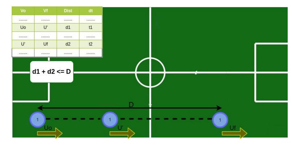
For one straight line, with a particular destination Pf and a target velocity Vf, as well as a start point Po and a initial velocity Vo, the algorithm need to find a maximum intermediate velocity V' such that the following expression is satisfied:
$$Dist(V_o -> V') + Dist(V' -> V_f) \le D$$
Where D is the length between Po and Pf and Dist(Va− > Vb) is the total distance traveled from going to Vb, starting from Va.
After calculating V', this value will be sent to the robot by the communication. V' is the maximum velocity that can be sent to the robot in order to achieve the closest point to Pf, with velocity Vf. It is important to mention that this calculation is performed at each point of the trajectory, so the value of V' will constantly change as the robot gets closer to Pf. Figure 1 shows an example for an initial velocity Uo and a final velocity Uf, the start point and the destination are separate by a distance D.
When there is more than one straight line, and just one target velocity for the end point of the last line, the same procedure is used to calculate the initial velocity of each line, starting from the last to the first. It is important to highlight that V o^n = V f^(n−1). The transitions are made, smoothly, by using a circle instead of a line, when the robot is close to the transition point.
2.1.3 Normal velocity
Finally, the angular velocity calculation is a simple PID controller. The orientation will be maintained aligned with the trajectory and will only change when the robot is closed to its target. As mentioned above, the values from the tables are just for tangential velocity, when the robot is not aligned with the trajectory, the velocity vector found, that has direction aligned with the trajectory, is decomposed in the normal and tangential component with respect to the orientation of the robot. The normal velocity has a maximum threshold, when is greater than it, the resultant direction of the velocity is maintained, the normal component will be the maximum possible and, then, the tangential velocity will be already defined.
It is important to notice that we are not handling acceleration constraints that can cause slippage. We prevent this by drastically reducing the maximum velocity in the normal direction and keeping the robot aligned to the trajectory. This is a limitation that we are currently working on for RoboCup 2022.
2.2 New kick logic
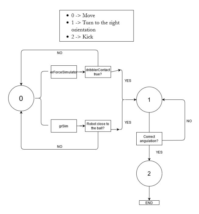
To improve the robot's kick skill, a new logic was made focusing on adding the dribbler function, in order to make plays like passing the ball more effective. The main reason to work on a new logic for the kick was to reduce the time to kick or pass the ball. In contrast to the old logic, which made the robot go to behind the ball and just after that, kick it, the new one uses the dribbler to make it faster, now the robot doesn't need to make all this process mentioned. To be specific, in this logic, a state machine was developed with three states:
- Move: The robot is oriented to the ball and goes to its coordinates until reaches a desirable distance from it, one close enough to be able to touch the ball. While the distance isn't the desired one, the robot keeps repeating the analysis in this state, which is checking the distance from it to the ball.
- Turn: Now that the robot can touch the ball, the dribbler function is activated and the robot turns with the ball to the desired orientation, which is the target direction, using a range of orientation to give a good precision for the kick. Therefore, while the robot's orientation isn't in this range, it keeps turning.
- Kick: After fulfilling the two states before, the robot can kick the ball to the target.
The diagram of the process can be seen in figure 2.
The logic was developed to work on two simulators, GrSim and erForceSimulator, making use of the dribblerContact boolean, present on both, which is a better choice to analyze the transition from the move state to the turn state based on the tests realized. In particular, when we are using the dribblerContact boolean we are preventing cases like the robot turns without the ball, event that used to happen when just the distance from the ball was analyzed. Due to this implementation the transition beet wen "Move" and "Turn" started to be more accurate.
If the dribbler sensor's performance is bad, we will replace it with two logics that are still in development and we believe are ready by RoboCup:
– FastKick: This strategy is focused on the passing strategy, which can be used for the shot on goal. It positions the pass receiving robot at an angle that
- allows a direct shot to a target (allied robot or Goal) without the need to stop the ball. In this type of strategy, it would not be necessary to use the dribbler.
- FastReturn: This strategy seeks to make curved trajectories so that the robot is behind the ball without the need to go too far back and then go forward, which was necessary due to the low confidence of the old control model.
2.3 New attack strategy
During the last competition we noticed that our robot team had few opportunities to attack, as there were almost always 3 robots in defense and 2 in attack. So, looking for a quick and simple solution for this, we created the new attack strategy, which follow certain criteria:
- Ball possession is ours.
- Command other than Stop, Halt and Timeout.
- Ball on the field.
- Must satisfy the startup conditions.
This strategy, in particular, uses existing positions from past competitions and controls up to a maximum of all robots except the goalkeeper, as the maximum number of current robots on the field for our team is 6, we calculate 5 possible positions, and them choose the robots available in order to optimize positioning in the field and reduce unnecessary movements.
As these plays were created with the idea of bringing simplicity to the code, we realized that during ball possession it is not necessary to separate the team in defense and attack, as the robots must be prepared to receive a pass or kick into the goal.
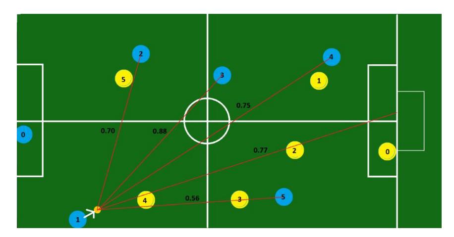
Thus, in every interaction of possession of the ball, a coefficient called FactorPass is calculated, which aims to provide how likely the ball will reach a goal starting from the robot closest to the ball, having a value between 0 and 1, resulting from a weighted average where the weights are obtained manually, and the criteria also vary from 0 to 1, a example of the coefficient is shown in Figure 3.
During the game, the objectives that use this factor are:
- Pass ball from one robot to another with the following criteria:
- Possible ball interception during the path from one robot to another.
- Dangerous robots behind the receiver that can steal the ball.
- Possibility of kicking the receiver's goal.
- Distance from receiver to goal in relation.
- Kick the ball into the goal, with the following criteria:
- Possible ball interception during the path from one robot to another.
- Risk of the goalkeeper's defense.
- In this strategy, there are four possible states:
- Default state: This state will be start if none of the other state are started, keeping a robot towards the ball, while the others are stationary, if during 450mm to 250mm from the robot to the ball, the pass state is not started this robot will kick directly into the goal.
- Prepare pass state: This state will be start if the referee's command is prepare direct, placing a robot close to the ball and distributing the others on the field.
- Keeper state: This state will be start if the ball enters our goal area, distributing the robots on the field.
- Pass state: This state will be start when the FactorPass of any allied robot is superior to the kick on goal. In this sense, the robot that has possession of the ball will give the pass to the robot with the highest coefficient.
2.4 Replay button
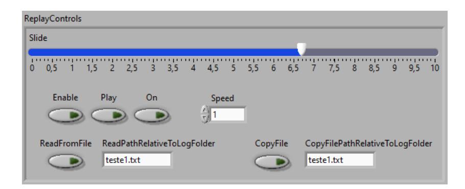
A real-time replay was implemented in our code to provide fast and easy debugging and game analysis, without the need to start recording game logs previously. The features and controls for this replay can be seen in detail in figure 4.
The replay feature works by storing each vision packet, as well as its corresponding timestamp to a ring buffer with length equal to a predetermined number of frames. So, when we fill the entire buffer, the oldest values will be overwritten, maintaining a window of fixed size. To further improve debugging, we can also save additional information that is stochastic or may vary between different runs with the same data, like the path generated by the path planning.
To replay the data, we place the cursor shown in figure 4 in the time position that we want, after hitting the play button, data will start to be fetched to our software, the time delay between each frame will be determined by the timestamps that were previously stored.
In our interface, there are three buttons: Enable, Play, and On, as well as speed control and special commands to save and load replay data from files.
The Enable button turns on writing data to the buffer, the On button is for starting/stopping the replay, and finally, the Play button pauses/continues the simulation at the cursor's current position, fetching the same frame multiple times in the pause state. Additionally, the speed control increases or decreases the time stamp difference between frames, giving the impression of a faster or slower simulation.
Currently, there are other log tools available to use, but we prefer to implement a solution completely integrated into our software. The main reason is that it's easier to debug, anytime the user wants, it can pause the code and go backward some frames, replay again and change simulation speed, without the need to save and play game logs previously. The other two reasons are the ease to add new features that just make sense to our code, and the possibility to replay custom data, like it was said previously about the path planning, for example.
3 Electronics Project
For RoboCup 2022, our team comes with a new project with major changes in hardware and firmware. The changes in the boards design were made based in the new motors, new battery and the new dribble system. The motors used in the previous robot model had their production discontinued what led to a replacement by GB37Y3530-12V-251R and also the battery replacement by LB3300LB3. Despite the range of necessary modifications, new additions and improvements made in the project, the modularization was preserved, carrying the previous models technologies in the 2022 model.
3.1 Firmware
Our robot's firmware uses an object-oriented programming architecture, written in the C++ language and the STM32CubeIDE development environment. This year's changes include a complete code remake, using the STM32 HAL library, an USB debug option, a new RF24 library coded by our team and the necessary modifications to interface with the new motherboard and the new peripherals, like the OLED display. This makes possible the addition of a new telemetry system that allows checking robot status, speed, battery voltage and sensor readings during the game without the need for a timeout. Also, the code is written using better practices than the previous one, making it easier to debug and add new features in the future.
3.1.1 Robot Communication
Modifications in the communication allowed the implementation of a bi-directional link system. This change makes possible to receive feedback from sensors, improving its interpretation by the AI, looking for fixing package loss issues and making debugging easier. The feedback packages include battery charge, wheels speed, ball possession, kicker charge, gyroscope readings and current measurements from critical parts of the circuit.
3.2 Control
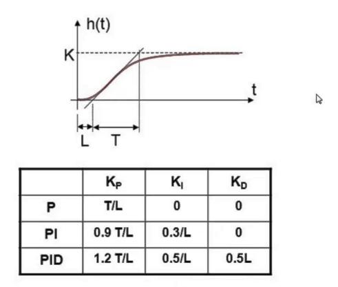
The electronic control uses a closed loop algorithm that is fed by the data generated by the encoder. We use an PID controller and the Ziegler–Nichols's method of obtaining PID constants. We noticed that Control was one of the biggest issues observed in latter versions, therefore big changes were made in the way calculations, data filters and signal generations are made in the firmware. In addition, the motor and the encoder were changed in order to improve our robot speed and velocity readings.
Furthermore, the method of obtaining PID constants has been improved using bench testing to study the step response of the new motor. Those modifications focused in making the movement more stable and the responses to errors and trajectory corrections faster. Related to controlling issues, the motor themselves were a problem in older projects, since they were bought in different years and used for different times, they presented different responses to the same input. Therefore, a measure taken to prevent those kinds of issues was the acquisition of all the motors from the same batch to guarantee a similar output to the same entry signal.
3.2.1 Ziegler–Nichols's method
The Ziegler-Nichols rule is a heuristic PID tuning rule that attempts to produce good values for the three PID gain parameters: Kp, Ti and Td, given two measured feedback loop parameters derived from measurements: Tu (the period of the oscillation frequency at the stability limit) and Ku (the gain margin for loop stability), with the goal of achieving good regulation (disturbance rejection).
3.3 Board Designs
The new boards design was created based in the 2018 /2019 version and adjusting the necessary parameters, since the change of battery and motors have required a new mother board and motor modules.
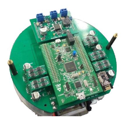
3.3.1 Stamp module
The module is the STM32F407 – Discovery, a development kit that includes an Arm Cortex M4 and other peripherals sensors, USB plugs, debugging LEDs, push buttons, motion sensors and others. This module is responsible for performing calculations and coordinating the signals sent and received from the different parts of the robot, like motor drivers, kicker module, communication board and sensors.
3.3.2 Main Board
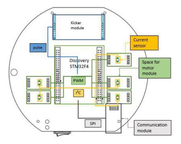
The Main Board (see figure 7) provides physical support to the modules and the connections between them and the robot's actuators, sensors and power supply. Most of the main board is composed of simple routes and planes that make these connections. It also implements some important circuits, such as the currents that flow to the motors and the side circuitry for CI's.
The new board, 2021 model, is the successor of the 2018 board. This new version presents significant changes with respect to its predecessor. About the changes, the motor internal circuit received the addition of a tension regulator of 3.3V in series with a 100K resistor as well as the replacement of the 1K ohm resistor for one with 15K ohm of resistance. There was also the addition of a power switch and the replacement of a 7 segments display by a new A2C led display.
3.3.3 Motor module
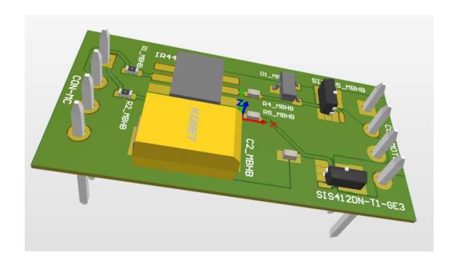
A new motor module was designed to be able to deliver the maximum power that the new motors may demand, maintaining the same pinout as its older version to keep the modularity of the project. As the motor that used to drive the wheels in past versions of the robot is no longer manufactured, we were forced into updating the robot's movement. We weren't able to find a replacement that could deliver a similar power output to the same input and therefore we had to make greater updates to the whole robot to change the operating voltage to 12V. The main changes to make this happen was, of course the battery, and also the motor module that consists in a H bridge that drives the motor. The new version is able to deliver more power than the last one without overheating and operating in a more reliable range, further away from the operation limits of the components.
3.3.4 Kicker module
The kicker module was maintained as the same as its older version since it's capable of delivering fair results in the new project version.
4 Mechanical Project
The mechanical project suffered some changes compared to the previous year's version. Currently, the team is focusing on improving not only the robot's efficiency and robustness, but also the ease of maintenance. With this in mind, RoboIME is constantly seeking new solutions for the project and through much research and information exchange with other teams some changes were made in the mechanical project. Below, are described the developments and the planning for RoboCup 2022.
4.1 New Motors
For 2022 we made a change in our motors. We now will use 12 Volts motors that will provide for the dribbler and for wheels. Both of the motors now came from factory with a magnetic encocder, although the dribbler encoder will not be consider on the game, this change will permit us to test in our labs the best rotation to the dribbler, as well as more precise control of the moviments of the robots.
4.2 Omni Wheels
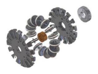
The robot's omni wheels have been completely modified. The main objectives of this change were to ease the robot's maintance and reduce costs. The omni now features a single layer of 15 small wheels each (see figure 9) and your diameter was modified from 35 mm to 45 mm. The use of a bigger wheel combined with the new motors will provide more speed to the robot. The body of the omni wheels will be printed, what will reduce our costs and the wheight of the robot.
4.3 The Kick System:
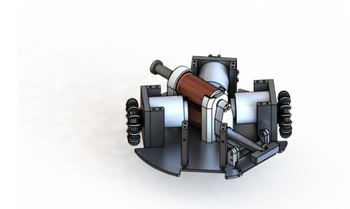
- Low Kick: The low kick was designed to pass by the high kick plate, in order to optimize the low kick performance. This system consists of a cylindrical solenoid, a piston which has the same geometry, a spring on one of the edges of the piston and the low kick plate on the other edge. While a current is passing through the solenoid, the piston goes ahead and then the low kick plate hits the ball. This movement stretches a spring and when the current finishes, the spring pushes the piston back again.
- High Kick: The high kick system has the same activation as the low kick system, but with some differences. The high kick was created to use the superior part of the robot and its kick plate was designed to pass under the low kick one. The piston moves and hits a little plate, which has a ramp on its front. This ramp was designed to cause the ball to move upward.
- The two systems have the same activation and piston geometry in order to make the analysis and the modeling simpler.
4.4 Battery Holder
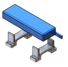
The battery holder consists of a mechanism which can hold the battery in a specific place. Besides that, it needs to be easy to handle, that means it has to be easy to be placed and removed.
In the modeling, it was kept the best geometry to permit accessibility and not let the battery free to move when the robot moves around. This project so simple,it is basically made of a battery compartment and two velcro strips that keep it pressed and prevent it from leaving the holder. Therefore, it helps to maintain the battery at the desired position (See figure 11).
4.5 Motors Fixture
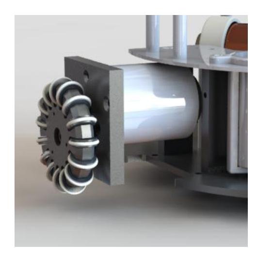
Due to hardships in previous competitions to make in-game maintenance of the motors, the fixture of the motor's assembly was redesigned to have an easyswap assembly. Previously, it was required to disassemble the entire first floor to access the motors. Now the whole subassembly of the motors can be detached by removing the screws on the side of its walls, much more accessible as shown in the figure 12.
4.6 Planning for RoboCup 2022
For Robocup 2022, new robots are going to be assembled without reusing parts from the robots that are already assembled. However, for the current RoboCup, some robot parts that were made of plastic through 3D printing will be made of metal to increase the robustness and durability of the robots.
5 Conclusions
For this competition, the aim is to consolidate the progress made in the previous years, experimenting with changes in the software project allied to the new electrical and mechanical project.
To summarize the important changes described by this paper, we can cite some important changes in each area. First of all, our software was improved by developing a new Navigation algorithm, a new Kick logic, and a new Attack strategy. In electronics, besides the firmware improvement, we had also to update the design of the Main Board and Motor modules in order to change motors. Finally, the new mechanical project (also designed to adapt for the new motors) included the new Omni Wheels, the improvement of the Kick System, and better positioning for battery and motors.
By applying these features, we should be able to perform better plays and get great results at RoboCup 2022 tournament.
5.1 Acknowledgement
This research was partially supported by the Army's Department of Science and Technology (DCT), Funda¸c˜ao Carlos Chagas Filho de Amparo `a Pesquisa do Estado do Rio de Janeiro - FAPERJ(grant E-26/111.362/2012); F´abrica de Material de Comunica¸c˜ao e Eletrˆonica (FMCE/IMBEL) and the IME alumni association. Special thanks to all former members of RoboIME. Without their support, this team would not be here.
References
- Gabriel F. Santos Felipe W. V. da Silva Antˆonio S. G. Pereira Erick T. da Silva. Leonardo G. Gon¸calves Lucas B. Germano Lucas G. Corrˆea Henrique Barreto Mayara R. Mendon¸ca Pedro Henrique Marques Isabel C. de Freitas Davi H. M. Pontes Luciano de S. Barreira Luis D. P. de Farias Jo˜ao G. O. C. de Melo Matheus Bozza Matheus P. de Souza Nicolas S. M. M. de Oliveira Onias C. B. Silveira Rebeca P. dos Reis Yugo Nihari Gabriel H. M. Silva Guilherme M. Gon¸calves Gustavo C. K. Couto Vinicius de F. L. Moraes Luis R. L. Rodrigues Carla S. Cosenza, Gabriel B. da Concei¸c˜ao and Paulo F. F. Rosa. Roboime larc 2020: A virtual challenge. pages 1–6. Available at https://github.com/roboime/roboime-tdp.
- Gabriel B. da Concei¸c˜ao Felipe W. V. da Silva Antˆonio S. G. Pereira Gabriel T. Pinheiro Gustavo A. Testoni Davi H. M. Pontes Daniel S. C. Bello Ana C. A. Monteiro Jos´e L. de O. Schramm Gustavo C. K. Couto Leonardo G. Gon¸calves Lucas B. Germano Luiz R. L. Rodrigues Guilherme M. Gon¸calves Vinicius de F. L. Moraes Gabriel H. M. Silva Mayara R. Mendon¸ca Ana L. B. da Silva Matheus Bozza Luis D. P. de Farias Jo˜ao G. O. C. de Melo Nicolas S. M. M. de Oliveira Lucas G. Corrˆea, Carla S. Cosenza and Paulo F. F. Rosa. Roboime: From the top of latin america to robocup 2020. pages 1–21. Available at https://github.com/roboime/roboime-tdp.