RoboDragons 2023 Extended Team Description
Masahide Ito, Marina Shibata, Shinjitsu Agatsuma, Yuta Ando
School of Information Science and Technology, Aichi Prefectural University
https://robodragons.github.io/
Abstract RoboDragons are a team of the RoboCup Soccer Small Size League (SSL) from Aichi Prefectural University, Japan. In RoboCup 2023, they will use the seventh-generation robots—developed in 2016 for the SSL competition. This paper shares the technical information of system updates implemented between 2022 and 2023: a new omni-wheel from the hardware part and an angular velocity controller of wheel motors from the software part.
Introduction
RoboDragons are a team of Aichi Prefectural University (APU) participating in the Small Size League (SSL) of RoboCup Soccer. This team originated from Owaribito—a joint team between APU and Chubu University—which was founded in 1997. In 2002, since two universities have been ready to manage each individual team, APU built a new team, RoboDragons. After that, RoboDragons have been participating in the SSL for more than 19 years including activities as CMRoboDragons—a joint team with Carnegie Mellon University in 2004 and 2005. Our best record was the second place in 2009. We also finished thrice in the third place (2007, 2014, and 2022) and four times in the fourth place (2004, 2005, 2013, and 2016). In RoboCup 2022, we placed third out of five teams in Division A.
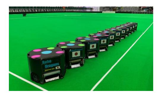
Similarly to last six years, the seventh-generation (7G) robots (Fig. 1), which developed in 2016, will be used in RoboCup 2023. For this generation, the first official matches were in RoboCup 2017. See our ETDP 2017 [1] for its hardware and software specification. After that, based on the issues found in some official/friendly matches and daily development, we have tried to improve the hardware and software.
From 2017 to 2018, to widen the ball-touchable area of the dribbling roller, some spaces on the side brackets of the dribbler were whittled down; to improve motion control of the robots, a trajectory tracking controller based on Model Predictive Control (MPC) [2] was developed [3]. From 2018 to 2019, the smalldiameter wheels around the omni-wheel were replaced for their more smooth mobility and less maintenance; to increase the successful rate of ball placement starting near the wall even if the dribbler does not work for keeping the ball, a skill to kick a ball to the wall diagonally was added [4]. From 2019 to 2020, to improve the dribbler so as to keep the ball more, different kinds of rollers were evaluated; a local vision system and control algorithm for SSL-Vision Blackout Challenge were developed [5]. From 2020 to 2022, our MPC-based trajectory tracking controller was upgraded so as to improve obstacle avoidance performance [6].
This paper provides the technical information of system updates that RoboDragons have implemented between 2022 and 2023. In the hardware part, our new omni-wheels developed for smooth driving under a reasonable cost are introduced; in the software part, a wheel motor controller for improving transient and steady-state responses of its angular velocity is presented.
Hardware Update—Design of New Omni-Wheels
In 2019, the small-diameter wheels on the omni-wheels have been replaced with smoother travel and less maintenance [4]. Most of the small-diameter wheels, however, were damaged from 2020 to 2021. The reason can be that the Nitrile Butadiene Rubber (NBR) tire baked on the A2017 hub could not withstand against the force applied tangentially to its circumference and then it was peeled from the hub. Between 2021 and 2022, the omni-wheels were completely redesigned and updated.
The basic structure is the same as in [7], which means that a silicone rubber tire and a plastic hub are put together and those parts are sandwiched by stainless steel washers. To reduce the cost, the small-diameter wheels were composed of ready-made silicon tubes and metal parts. As a result, the thickness of the small-diameter wheel was increased, so the base and cover parts had to be newly redesigned. Fabricating them by cutting aluminum as before would cost high in terms of time and budget. In addition, trial and error are required for designing and prototyping. We therefore decided to shift to fabrication using a 3D printer.
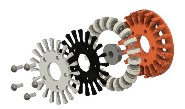
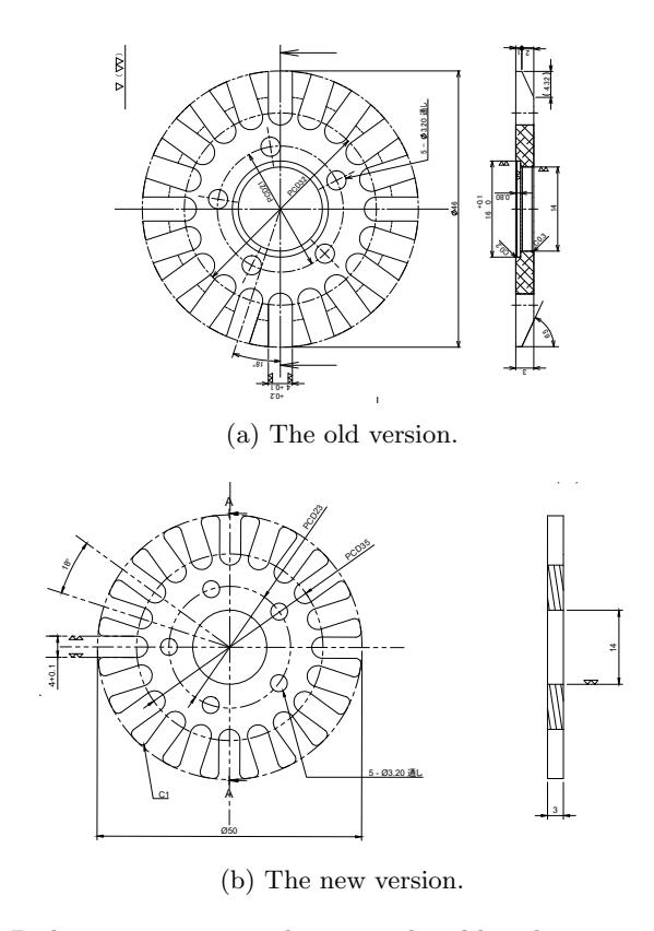
The key points of the design are as follows (Fig. 3):
- To achieve both strength and low cost, ABS resin—which is stronger than PLA resin—was chosen for the base part;
- The cover part made of A6061 aluminum alloy was 1 mm thicker than the previous one of 3 mm in consideration of contact/collision with other robots.
- To reduce the cost and ease of machining, the design was simplified by eliminating the cutting and grooving of the hold section, and also the material was changed from A7075 to A6061.
Owing to the above-mentioned design changes, the fabrication cost per a omniwheel has been reduced to one-fifth of the previous one.
As a tire of the small-diameter wheel, two types of silicon hardness—A70 and A90—were compared. A robot using the A90 tire tended to result in error in the position control. This is because the tire slid when the robot accelerated or decelerated due to low friction with the carpet caused by the hardness of the silicon. On the other hand, the A70 tire has almost no difference in running performance compared to the previous one.
The developed omni-wheels were deployed in RoboCup 2022 and JapanOpen 2022. During those competitions, the omni-wheels did not break significantly and no parts fell off. After the competition, however, deformation was found in some of the cover parts. For such deformation, there are two possible reasons:
- The base part made of resin is soft. When the robots collide with each other or receive an external shock, the soft base dents to absorb the shock;
- The cover part is made of A6061, which is a relatively soft material among aluminum alloys.
Based on above-mentioned inference, there is an idea to improve our omniwheel further, which is to insert a cushion of highly flexible TPE (Thermoplastic Elastomers) resin between the cover and base parts to absorb the shock received by the cover (Fig. 2). This further-improved omni-wheel will be used in RoboCup 2023, and its durability and running performance will be evaluated through competitions.
Software Update—Angular Velocity Control of Wheel Motor in Consideration of Disturbance
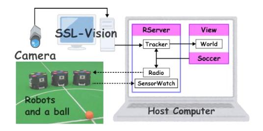
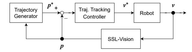
The fast-paced soccer in the SSL is provided by a combination of a global vision system (called as SSL-Vision), wireless network, omni-directional mobile robots, and a centralized system as depicted in Fig. 4. In particular, the basic performance of each team depends on their motion controller. As introduced in [6], RoboDragons adopts a two-layered control system: the upper-layer controller (Fig. 5(a)) is for trajectory tracking control of the robot; the lower-layer controller (Fig. 5(b)) is for angular velocity control of wheel motors.
Regarding the upper-layer controller, RoboDragons have developed MPC-based trajectory tracking controllers [3,6]. Refs. [3,10] proposed the controller in consideration of limitations of robot's linear velocity and acceleration. Additionally, in [11,6], it was extended so as to enable obstacle avoidance.
On the other hand, the lower-layer control system (Fig. 5(b)) is running onboard based on the velocity command provided from the upper-layer controller. The velocity command with respect to the robot itself is transformed into the one with respect to the wheels through the inverse kinematics derived from the mechanical structure. At each wheel, the actual angular velocity is followed to the command via a feedback controller so that the robot realizes the desired behavior finally. This ETDP will share the information about our angular velocity controller of wheel motors in consideration of disturbance.

Angular Velocity Controller in Consideration of Disturbance
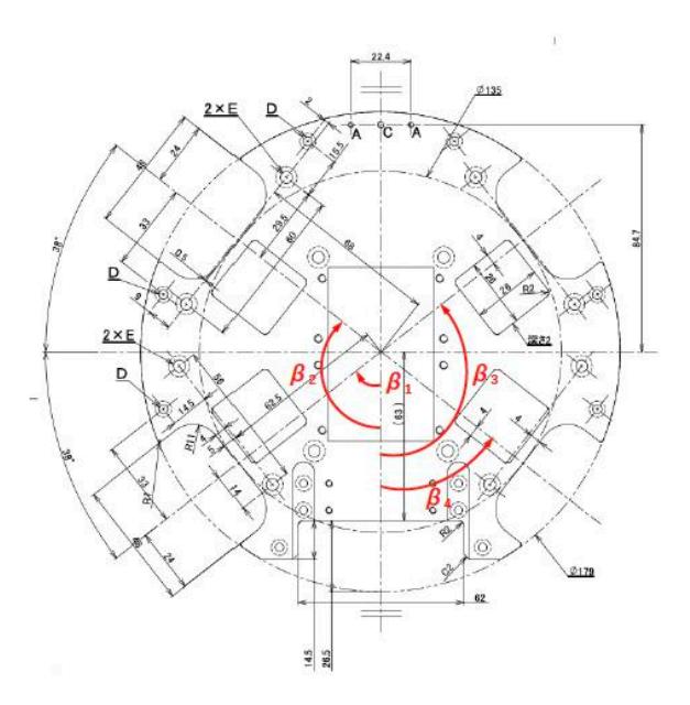
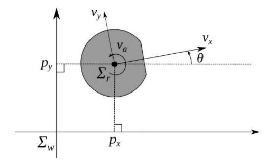
Table 1 summarizes parameters of the motor and wheel. As shown in Fig. 6, four omni-wheels are aligned by angle $\beta_i$ with respect to the front (i = 1, 2, 3, 4). The robot velocity command $\mathbf{v}^* := [v_x^, v_y^, v_a^]^\top$ (Fig. 7) is converted to the angular velocity command $\boldsymbol{\omega}_m^ := [\omega_1^, \omega_2^, \omega_3^, \omega_4^]^\top$ for the wheel motors by using the following relationship (inverse kinematics):
$$\boldsymbol{\omega}{m}^{\star} = \frac{\eta}{\frac{d{w}}{2}} \begin{bmatrix} \cos \beta_{1} & \sin \beta_{1} & -d \ \cos \beta_{2} & \sin \beta_{2} & -d \ \cos \beta_{3} & -\sin \beta_{3} & -d \ \cos \beta_{4} & -\sin \beta_{4} & -d \end{bmatrix} \boldsymbol{v}^{\star}, \tag{1}$$
where d is the distance between the wheel and robot's center.
A mathematical model of a DC motor can be represented by
$$J\dot{\omega}{mi}(t) + \mathcal{B}i \omega{mi}(t) = K{\text{PWM}} D_i(t), \tag{2}$$
where $J := J_m + J_p + J_w/\eta^2$, $\mathcal{B}i := B_i + K\tau K_{bi}/R$, and $K_{\text{PWM}} := K_\tau V_o/(200R)$, respectively. Parameters $B_i$ and $K_{bi}$, which compose $\mathcal{B}i$, are the viscous friction coefficient and back electromotive force (EMF) constant, respectively. In general, these constants are unknown and have to be identified from some experimental data. Meanwhile, the competition fields of the SSL—which are almost even surface at the beginning—have uneven spots through several matches. Those spots that slightly disturb the robot motion. Suppose that an external force $\tau{\text{ext}}$ is exerted into (2). Then, the following model can be considered instead of (2):
$$J\dot{\omega}{mi}(t) = K{\text{PWM}}D_i(t) - \underbrace{\left(\mathcal{B}i\omega{mi}(t) + \tau_{\text{ext}}(t)\right)}_{w_i(t)},\tag{3}$$
Now let's consider the second term on the right-hand side as a disturbance $w_i(t)$. By letting $x_i := [\omega_{mi}, w_i]^{\top}$, $u_i := D_i$, and $y_i := \omega_{mi}$ be a state vector, control input, and output, respectively, the model (3) can be described in the following state-space representation:
$$\frac{\mathrm{d}}{\mathrm{d}t} \boldsymbol{x}{i} = \begin{bmatrix} 0 & -\frac{1}{J} \ 0 & 0 \end{bmatrix} \boldsymbol{x}{i}(t) + \begin{bmatrix} \frac{K_{\mathrm{PWM}}}{J} \ 0 \end{bmatrix} u_{i}(t), \qquad (4a)$$
$$y_{i}(t) = \begin{bmatrix} 1 & 0 \end{bmatrix} \boldsymbol{x}_{i}(t). \qquad (4b)$$
Note that $x_i$ is the two dimensional vector. Meanwhile, the observability matrix is computed as follows:
$$\bm{M}_o \coloneqq \begin{bmatrix} \bm{c} & \bm{cA} \end{bmatrix} = \begin{bmatrix} 1 & 0 \ 0 & -\frac{1}{J} \end{bmatrix}.$$
Hence, rank $M_o = 2$, which means that the system (4) is observable. Now the following full-state observer can be used to estimate the state vector $x_i$ including disturbance $w_i(t)$:
$$\frac{\mathrm{d}}{\mathrm{d}t}\hat{\boldsymbol{x}}{i} = \boldsymbol{A}\hat{\boldsymbol{x}}{i}(t) + \boldsymbol{b}\boldsymbol{u}{i}(t) + \boldsymbol{h}(y{i}(t) - \boldsymbol{c}\hat{\boldsymbol{x}}_{i}(t)), \tag{5}$$
where $\mathbf{h} \coloneqq [h_1, h_2]^{\top}$ is the observer gain vector, which means that the estimation error $x_i - \hat{x}_i$ converges to zero if the observer gain vector h is appropriately chosen so as to assign stable poles. In particular, the estimated disturbance $\hat{w}_i$ is obtained by
$$\hat{w}_i(t) = \begin{bmatrix} 0 \ 1 \end{bmatrix} \hat{x}_i(t). \tag{6}$$
Next, by using the estimated disturbance (6) with (5), let's consider to design an angular velocity controller with a disturbance compensator. In order to follow the angular velocity command $\omega_{mi}^{\star}$, the following proportional-integral (PI) feedback controller with the derivative command feedforward and disturbance compensator is designed:
$$D_{i}(t) = \frac{1}{K_{\text{PWM}}} \left{ J \left( K_{P} e_{i}(t) + K_{I} \int_{0}^{t} e_{i}(\tau) d\tau + \dot{\omega}{mi}^{\star}(t) \right) + \hat{w}{i}(t) \right}, \quad (7)$$
where $e_i := \omega_{mi}^* - \omega_{mi}$. Applying the controller (7) into the system (3), the closed-loop system is expressed as
$$J\dot{\omega}{mi}(t) = J\left(K_P e_i(t) + K_I \int_0^t e_i(\tau) d\tau + \dot{\omega}{mi}^{\star}(t)\right) + \hat{w}_i(t) - w_i(t).\tag{8}$$
If $\hat{w}_i$ converges to $w_i$ quickly and enough, then the closed-loop system (8) can be considered as
$$\dot{\omega}{mi}(t) = K_P e_i(t) + K_I \int_0^t e_i(\tau) d\tau + \dot{\omega}{mi}^{\star}(t)$$
$$\Leftrightarrow \underbrace{\dot{\omega}{mi}^{\star}(t) - \dot{\omega}{mi}(t)}_{\dot{e}_i(t)} = -K_P e_i(t) - K_I \int_0^t e_i(\tau) d\tau. \tag{9}$$
Moreover, introducing
$$z_i(t) \coloneqq \int_0^t e_i(\tau) , \mathrm{d}\tau,$$
the closed-loop system (9) is reduced to
$$\frac{\mathrm{d}}{\mathrm{d}t} \begin{bmatrix} e_i(t) \ z_i(t) \end{bmatrix} = \begin{bmatrix} -K_P & -K_I \ 1 & 0 \end{bmatrix} \begin{bmatrix} e_i(t) \ z_i(t) \end{bmatrix},\tag{10}$$
which implies that the system (9) (or (10)) can be stabilized by setting gains $K_P$ and $K_I$ appropriately so as to assign stable poles.
Parameters of Motor and Wheel
| Symbol | Description | Definition or Value |
|---|---|---|
| $\beta_1$ | alignment angle of the first wheel | $-(38/180)\pi \mathrm{rad}$ |
| $\beta_2$ | alignment angle of the second wheel | $-(142/180)\pi \mathrm{rad}$ |
| $\beta_3$ | alignment angle of the third wheel | $-\beta_2$ |
| $\beta_4$ | alignment angle of the fourth wheel | $-\beta_1$ |
| $J_m$ | rotor inertia | $135 \times 10^{-9} \mathrm{kg \cdot m}^2$ |
| $J_p$ | inertia of pinion gear | $(1/8) m_p d_p^2$ |
| $J_{\omega}$ | inertia of wheel | $(1/8) m_{\omega} d_{\omega}^2$ |
| $m_p$ | mass of pinion gear | $2.88 \times 10^{-3} \mathrm{kg}$ |
| $m_{\omega}$ | mass of wheel | $40 \times 10^{-3} \mathrm{kg}$ |
| $d_p$ | diameter of pinion gear | $11.5\mathrm{mm}$ |
| $d_{\omega}$ | diameter of wheel | $55\mathrm{mm}$ |
| $g_p$ | number of pinion gear teeth | 21 |
| $g_{\omega}$ | number of inner gear teeth | 64 |
| $\eta$ | gear ratio | $g_\omega/g_p$ |
| $K_{\tau}$ | torque constant | $2.54\mathrm{mNm/A}$ |
| R | terminal resistace phase to phase | $0.403\Omega$ |
Experimental Verification
The effectiveness of the designed controller is evaluated via some experiments with a real robot. The experiments were performed under the following setting:
- To obtain 1 kHz sampling data from the robot directly, the robot was operated while connecting the PC for logging via a cable;
- To observe the step response while connecting the PC via a cable, robot's motion was limited to pure rotation (i.e., $v_x^* = v_y^* = 0 ,\text{m/s}$);
- The designed controller—referred as "PI + FF contr. w/ dist. comp."—is compared with "P + FF contr.", "PI + FF contr.", and "P + FF w/ dist. comp.";
- For the fairness of experimental comparison, the battery level was between 50% and 60% and also the actual responses of the rear and right (RR) omni-wheel were focued on.
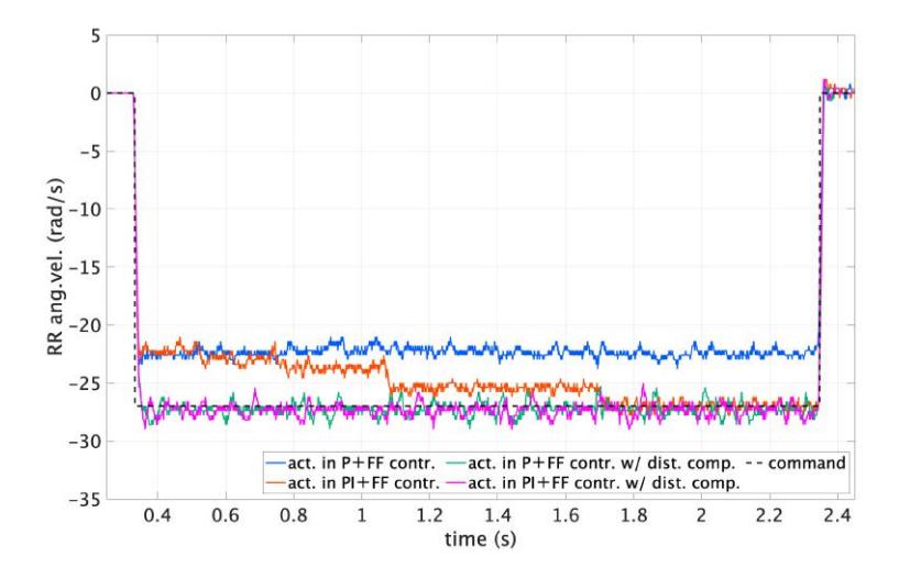
Figure 8 shows the experimental results performed with the following parameters: $v_a^{\star} = pi \text{ rad/s}$, $(K_P, K_I) = (6 \times 10^5, 1 \times 10^6)$ (i.e., poles are placed at $-3 \times 10^5 \pm 500\sqrt{359996}$ (< 0)), and $(h_1, h_2) = (300, -1.80 \times 10^{-2})$ (i.e., both poles are placed at -100), respectively. Note that experimental data was applied offline by centered 15-point moving average due to lack of encoder resolution.
From Figures 8, it can be observed as follows:
- The controllers with disturbance compensation have better performance, especially on the steady-state error, than the ones without disturbance compensation;
- Between the controllers without disturbance compensation, the response of "PI + FF contr." is better than that of "P + FF contr." The latter controller left the steady-state error while the former one compensates it over time (in about 1.5 s);
- There is no difference between the controllers with disturbance compensation, which may indicate that the I control is not necessary.
This result, however, is not bad because the SSL rules restricts the radius of an SSL robot to be less than 0.09 m. It implies that the radius of a virtual circular wall just has to be appropriately longer than the one of the real obstacle. Also, it can be seen that how much the robot invades the obstacle depends on the initial position. The reason is that the control problem considered here is setpoint regulation and also the initial position, i.e., distance between the initial and target positions, affects the acceleration of the robot near the obstacle.
Concluding Remarks
This paper has shared the technical information of RoboDragons 2023. In the hardware part, a design of a new omni-wheel for smooth driving under a reasonable cost was shown; in the software part, as for an angular velocity controller for improving the steady-state response was described.
Acknowledgement
The authors would like to thank Mr. Mizutani (OP-AmP, Japan) for his technical advice. The authors also would like to thank the other active RoboDragons 2022–2023 members, Ban, K. Kashiwamori, F., Yamada, M., Fujita, F., Sugiura, K., Suzuki, T., Kato, S., Kawada, J., Shimizu, T., Honobu, K., Miyazaki, Y., Mori, K., Iguchi, K., Kato, A., Nakayama, R., Nomura, H., Fujita, H., and Yuge, H. for their support.
References
- Adachi, Y., Kusakabe, H., Suzuki, R., Du, J., Ito, M., and Naruse, T.: "Robo-Dragons 2017 extended team description," RoboCup Soccer Small Size League, 2017. Available online: https://ssl.robocup.org/wp-content/uploads/2019/01/2017_ETDP_RoboDragons.pdf (accessed on 30 Jan 2023).
- Maciejowski, J.M.: "Predictive Control with Constraints," Prentice Hall, 2000.
- Ito, M., Kusakabe, H., Adachi, Y., Suzuki, R., Du, J., Ando, Y., Izawa, Y., Isokawa, S., Kato, T., and Naruse, T.: "RoboDragons 2018 extended team description," RoboCup Soccer Small Size League, 2018. Available online: https://ssl.robocup.org/wp-content/uploads/2019/01/2018_ETDP_RoboDragons.pdf (accessed on 30 Jan 2023).
- Ito, M., Suzuki, R., Isokawa, S., Du, J., Suzuki, R., Nakayama, M., Ando, Y., Umeda, Y., Ono, Y., Kashiwamori, F., Kishi, F., Ban, K., Yamada, T., Adachi, Y., and Naruse, T.: "RoboDragons 2019 extended team Description," RoboCup Soccer Small Size League, 2019. Available online: https://ssl.robocup.org/wp-content/uploads/2019/03/2019_ETDP_RoboDragons.pdf (accessed on 30 Jan 2023).
- Ito, M., Nakayama, M., Ando, Y., Adachi, Y., Du, J., Suzuki, R., Ono, Y., Kashiwamori, F., Ban, K., Isokawa, S., Yamada, T., and Naruse, T.: "RoboDragons 2020 extended team Description," RoboCup Soccer Small Size League, 2020. Available online: https://ssl.robocup.org/wp-content/uploads/2020/03/2020_ETDP_RoboDragons.pdf (accessed on 30 Jan 2023).
- Ito, M., Ando, Y.: "RoboDragons 2022 extended team Description," RoboCup Soccer Small Size League, 2022. Available online: https://ssl.robocup.org/wp-content/uploads/2022/04/2022_ETDP_RoboDragons.pdf (accessed on 30 Jan 2023).
- Goto, R., Asakura, T., Fujii, N., Matsuoka, K., Mizuno, M., Sano, T., Onuma, Y., Nagata, H., Watanabe, M., and Sugiura, T.: "KIKS 2013 extended team Description," RoboCup Soccer Small Size League, 2013. Available online: https://ssl.robocup.org/wp-content/uploads/2019/01/2013_ETDP_KIKS.pdf (accessed on 30 Jan 2023)
- Mattingley, J. and Boyd, S.: "CVXGEN: A code generator for embedded convex optimization," Optimization and Engineering, Vol. 13, No. 1, pp. 1–27, 2012. doi: 10.1007/s11081-011-9176-9.
- GVXGEN: Code Generation for Convex Optimization. Available online: https://cvxgen.com/docs/index.html (accessed on 1 Feb 2022).
- Suzuki, R. and Ito, M.: "Trajectory tracking controller based on linear model predictive control for omni-wheeled mobile robots with velocity command limits," Proceedings of the fifth IEEJ International Workshop on Sensing, Actuation, Motion Control, and OptimizatioN (SAMCON'19), Paper No. V1-7, Chiba, Japan, March 2019.
- Ando, Y. and Ito, M.: "Obstacle avoidance of omnidirectional mobile robots in consideration of motion performance," Proceedings of the seventh IEEJ International Workshop on Sensing, Actuation, Motion Control, and OptimizatioN (SAMCON'21), pp. 394–395, Chiba, Japan, March 2021.