RoboTeam Twente Extended Team Description Paper for RoboCup 2023

Jibbe Andringa, Thijs Bink, Brunon Bojkow, Jitka Bojorge-Alvarez, Hilke van den Born, Cas Doornkamp, Emy Ganzeboom, Umer Javed, Tom Meulenkamp, Emiel Steerneman

University of Twente (UT), Enschede, the Netherlands; RoboTeam Twente, Capitool 25 Enschede, the Netherlands

https://roboteamtwente.nl

Abstract RoboTeam Twente has participated in the Small Size League of the RoboCup for the previous six years. To help progress the current state of the competition the main innovations are outlined each year. This paper showcases the customised solenoids and new basestation. Additionally, this paper proposes a Machine Learning environment for play decision making, our improved path planning method, a standardised and extensible communication protocol for robots and their central computer, and an alternative/addition to the IR-based ball sensors that are used in most SSL robots.

1 Introduction

RoboTeam Twente is a multidisciplinary team consisting of students from the University of Twente and Saxion University of Applied Sciences. The team has been founded in 2016 by a group of students striving to challenge themselves in the fields of robotics and artificial intelligence. Now, six generations later, it is up to this year's team to improve the previous generations' design and further innovate on the current state of RoboTeam Twente's Small Size League (SSL) robots.

This paper will first discuss the changes made in the hardware in Section 2. Last years's extended team description paper (ETDP) [5] introduced a renewed modular design, which is further built upon this year. This is more elaborated on in Section 2.2. In this section, the strategy for optimising the handmade solenoids used in the robots are explained as well.

Section 3 will showcase the design for the new basestation, as well as describe the requirements that motivated the design.

Section 4 will cover the changes made to the robot's software. This section will include updates to the communication protocol, a detailed description of the plan to use machine learning for improved play decision-making, and an alternative to the existing infrared-based ball sensors used in most of the current generation SSL robots. A render of the robots described in this paper is shown in Figure 1. The robot's specifications can be found in Table 1.

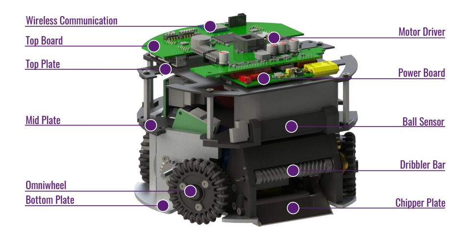
Render of the 2022 version of the robot.

Robot specifications.

2 Hardware

The hardware consist out of all the physical components of the robot. This is divided in mechanical and electrical parts. In recent years, RoboTeam Twente has been working on creating a more modular and robust design of the hardware. This year's team will continue on that path by focusing on fine-tuning the innovative ideas.

2.1 Electronics

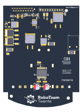
Since the electronics team of last year focused on a redesign of the existing PCBs with an emphasis on modularity, a complete redesign this year was not needed. Instead, research is dedicated to fine-tuning the modular designs to improve their accuracy, reduce the overall PCB footprint on the robot, and improve testing capabilities. Whereas traces and headers of several PCBs required relatively minor modification to support newer components, the kicker-and-chipper board required more research. The current design of the kicker-and-chipper board can be found in Figure 2.

Kicker-and-chipper board Over the past year, it has been discovered that the current iteration of the kicker-and-chipper board could not reliably charge the capacitor to its working voltage. Hence, further research was dedicated to the alignment of traces on the kicker-and-chipper board and improvements of the booster circuit.

The design of the current kicker-and-chipper board.

2.2 Mechanics

The mechanical overhaul of the previous generation has proven effective. For this reason, efforts of the current mechanics' team were dedicated to structural changes accommodating a new dribbler motor and chipper and to the optimisation of the solenoid.

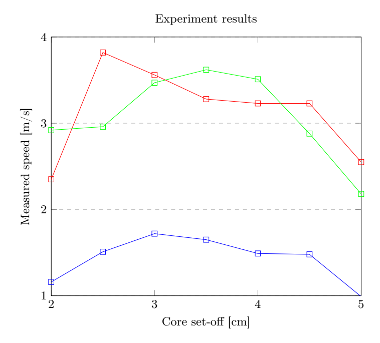
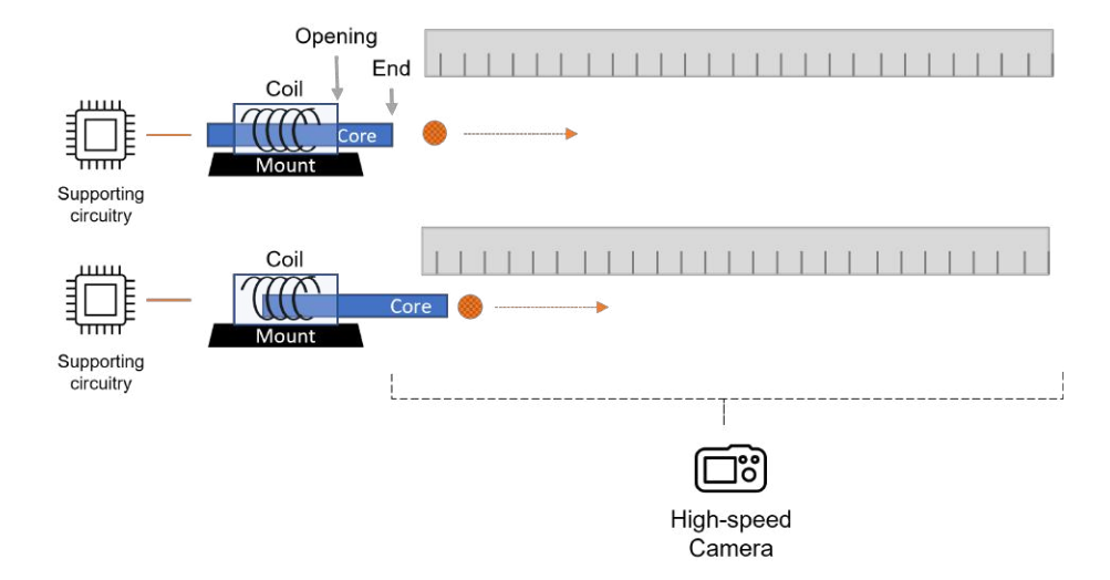
Solenoid performance is directly correlated to the placement of the core in relation to the coil. Through empirical research based on a series of experiments, the ideal placement of the core can be determined. Figure 4 shows the conceptual idea of the experiment setup in which the core's position can be adjusted. Solenoid-driven kicks of the ball were recorded in various positions using a highspeed camera, after which ball speeds were extracted.

The results of the experiment shown in Figure 3 (conducted with various configurations of the core and coil positions) have indicated that the optimal position of the end of the core with respect to the opening of the coil lies between 4.5 and 5.5 centimetres (see markings in Figure 4). It should be noted that results do vary for the different kicker-chipper boards that were tested, that is why every line indicates a different board

Based on the derived optimal core position, new fixtures (with hexagonal bearings and rods) were developed that simultaneously reduce the freedom of the rotational movement of the core.

Graph depicting ball speeds (of solenoid kicks) for different kicker-chipperboards with respect to the offset of the core in cm.

Conceptual drawing of the solenoid experiment setup.

3 Basestation

Some years ago, RoboTeam Twente started on the design of a new basestation as a side project. Previous and current designs consisted of a development board, such as an Arduino or STM32 Nucleo, connected to either an antenna or custommade antenna extension board. Earlier basestations lacked in performance and were quickly replaced. The currently used basestation held up for a couple of years, but is starting to show shortcomings with its hardware as the needs of the team started to grow. It is easy to forget about a relatively inconsequential piece of hardware such as the basestation. If it works, it works. However, without it, the robots are "nothing more than overengineered door stoppers" - Basestation Project Plan 2020-2021.

3.1 Shortcomings

USB limitations The data that needs to go through the basestation has grown with the years and with the introduction of REM. The data throughput limit and latency of the Full Speed (FS) USB connection, at 12 Mbit/s, is now a bottleneck. This is mostly due to the FS USB design with its 1 millisecond frame time. Because of this, packets to and from the basestation could be dropped as there were more packets per second than the FS USB connection could handle.

Power limitations The current custom-made antenna extension board features a connector to which a touchscreen can be connected, but the current needed to power the screen is too much for the USB powered Nucleo. It is possible to bypass the USB power by providing an alternate 5V source, but this is fault prone and needs frequent fixing.

Peripheral limitations An often requested feature is the possibility to log all traffic that goes through the basestation, as well as the status of the basestation. For this, an SD card is a possible solution. However, there is no way to connect it to the Nucleo.

3.2 Design

Figure 5 shows a rendering of the new basestation. In Table 2 one can find a list of features of this new basestation, where a ✓ indicates a feature that is new. This new basestation is designed around the STM32F767ZIT6 micro controller, same as the Nucleo and robots. The new basestation features more peripherals. For one, the USB is upgraded to a High Speed (HS) USB by using the USB3300 USB PHY chip through the ULPI interface. This increases the theoretical max transfer rate to 480 Mbit/s, from 12 Mbit/s as per USB FS. This upgrade makes the basestation USB 2.0 compliant, meaning that micro frames (125µs) are possible instead of the 1ms frames. This reduces the latency and increases the amount of individual packet transfers possible. The USB interface is now also split up between a high priority interface (RobotCommands and RobotFeedbacks) and a low priority interface for all other messages (debugging data, logging, etc). With this, there is now always enough bandwidth reserved on the bus to keep the main process running smooth, and all other messages are buffered and transmitted when possible.

The new basestation has two possible power inputs, 12V from a common 12V supply, or 12-24V from a LiPo battery. This allows the basestation to function continuously when stationary or from remote areas where no wall power is present. This, in combination with the touch screen, allows the basestation to be fully independent and portable for events and demonstrations. With these power inputs, the basestation now also requires only a single USB connection. The new basestation also features a high throughput SDIO connection to an SD card for logging purposes or saving settings between power cycles.

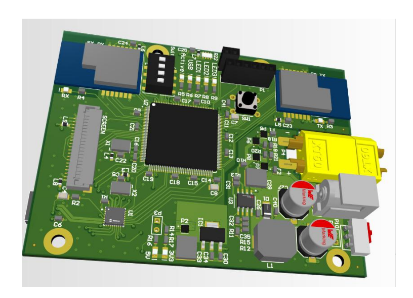
Features of the new basestation.

4 Software

Where last year's ETDP [5] was focused on the hardware, this year's paper will mainly be focusing on software. The team has been working on improving and standardising the communication between AI, basestation and robots. Additionally, the Artificial Intelligence that controls the robots is currently being trained with a Machine Learning model, in order to enhance the play decision making software. The controllers of the robots have received an updated structure, allowing for more consistency. Next to that, a proposition for an alternative and/or addition to the conventional Infrared(IR)-based ball sensor that is being used by most SSL robots nowadays is stated in this section.

4.1 RoboTeam Embedded Messages

As is the case with every team, the robots engage in wireless communication with the AI. In the first few years, two simple messages were going from and to the robot; a RobotCommand message and a RobotFeedback message. Both of these messages are basically a list of values. For a RobotCommand, think of e.g velocity, rotation, kicking, and chipping. For a RobotFeedback, think of velocity, rotation, battery level, and ball-sensor readings. Handwritten code (in C) was responsible for converting high-level objects (C structs, Protobuf messages, custom class instances, etc) into an array of bytes that represented these two messages. Since these messages should be compact to keep throughput high, this handwritten code involved a lot of bit-shifting and masking. It had to be written for both the computer and the robots. The problem with this is that code is error-prone, hard to read, and difficult to modify.

The solution In an attempt to solve this problem, more code was written (in Python) to auto-generate this C code, giving a definition of the message (in Python as well). The generator also generates Python files for quick development and prototyping. There are plans to generate Rust code, as well as Protobuf definitions. In Listing 1.1 is a small (stripped down) example to control a robot via Python as well as logging, using the pySerial library for communication with the basestation. All of the files can be found at the GitHub [9].

Listing 1.1. REM sample code.

1 import s e r i a l
2 import REM. python . REM_BaseTypes a s BaseTypes
3 from REM. python .REM_RobotCommand import REM_RobotCommand
4
5 command = REM_RobotCommand ( )
6 command . heade r = BaseTypes .
       REM_PACKET_TYPE_REM_ROBOT_COMMAND
7 command . pa yloa d Si z e = BaseTypes .
       REM_PACKET_SIZE_REM_ROBOT_COMMAND
8 command . ro bo t I d = 1
9 command . v e l o c i t y = 4
10
11 bits_and_bytes = command . encode ( )
12
13 b a s e s t a t i o n = s e r i a l . S e r i a l ( "/dev/ s e r i a l /by−i d /
        ba s e s ta tio n_1 " )
14 b a s e s t a t i o n . w ri t e ( bits_and_bytes )
16 with open ( " l o g .rem" , "wb" ) a s f i l e :
17 f i l e . w ri t e ( bits_and_bytes )

The evolution With the capability to quickly and simply generate code, came the desire to have more messages than just the aforementioned two. For example, there is now a RobotStateInfo message that contains detailed information such as individual wheel speeds and PID integral values. There is also a RobotMusic-Command message to control the speakers. These messages can be used while developing the robots, and turned off during a match. Over time, the number of different messages grew, and there are currently sixteen types. A new issue arose, where custom code had to be written to route and decode each type of message, even though it was mostly copy-and-paste work. To solve this, the messages were structured not unlike a TCP packet, where each message contains basic information regarding routing. This includes source and destination (robot, basestation, AI), protocol version, timestamp, and message size. While this slightly reduces flexibility in creating messages (since basic information is enforced), it greatly eases development. A bit-wise representation of this basic information can be found in Figure 6. Accompanying one can find the legend in Table 3.

The project can be seen as an amalgamation of TCP and Protobuf, borrowing features from both, resulting in faster prototyping, improved logging, and easier robot debugging and development. Using Python, engineers can test the entire robot with a simple script instead of installing the full software stack. The additional information allows control engineers to profile the robot and extract more insights by defining new messages.

Open Source The entire project can be found on GitHub [9]. Neither the generator nor the generated C code require additional libraries. The generated Python code requires Numpy.

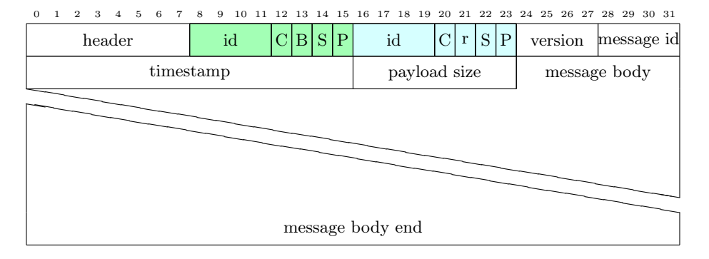
Packet legend.

Field	Description
header	The header byte, indicating the type of packet
id	The id of the receiving robot
C	The colour of the receiving robot, either yellow (0) or blue (1)
В	Whether this is a broadcast packet
S	Whether this packet is meant for the basestation
P	Whether this packet is meant for the PC
id	The id of the transmitting robot
С	The colour of the transmitting robot / basestation, either yellow (0) or blue (1)
r	Reserved
S	Whether this packet comes from the basestation
P	Whether this packet comes from the PC
version	The version of the protocol
message id	The id of this message, used for aligning packets
timestamp	The timestamp in milliseconds
payload size	The size of the payload. Max 255 bytes, including this header

4.2 Artificial Intelligence

The development of AI algorithms for RoboCup SSL robots poses a significant challenge due to the need for efficient testing and training. To address this, a new high-level simulator has been designed to improve the simulation process. The current low-level physics-based simulator (grSim [8]) is known to slow down the simulation significantly. The new high-level simulator allows for easy implementation of Machine Learning techniques, thereby enhancing the decision-making process. Finally, a new path planning algorithm will be proposed, which builds upon the existing path planning and enhances it by providing efficient collision avoidance while maintaining the fastest possible path.

High level simulator One important aspect of developing AI for RoboCup SSL robots is the use of high-level simulators. These simulators allow for the efficient testing and training of AI algorithms, enabling the development of more advanced and capable robots without the need for expensive hardware or realworld testing. In this section, a description of a high-level simulator for RoboCup SSL robots will be provided that is specifically designed for machine learning in play decision making.

Inspired by the built-in simulator from TIGERs [6], this simulator does not use a physics engine, instead it provides a simplified representation of the game state and the actions that the robot can take. This makes it more efficient for the training and testing of AI algorithms for decision making. The simulator includes a variety of tools and features that enable the efficient training and testing of AI algorithms for play decision making.

One of the key features of the simulator is its ability to generate a wide range of different scenarios, including various game states and opponent strategies. This allows the AI to be trained on a diverse set of situations, increasing its robustness and adaptability in real-world scenarios. Additionally, the simulator also includes a variety of performance metrics that can be used to evaluate the effectiveness of different AI strategies. This enables us to quickly test and iterate on different AI algorithms and fine-tune them for optimal performance.

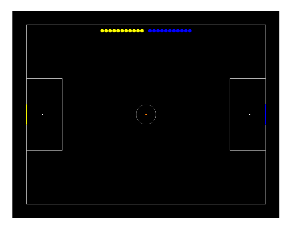
The proposed simulation utilises a step-based methodology, which allows for the pausing and progression of the game in both forward and backward directions. This approach provides significant benefits in terms of its flexibility and ease of use. Specifically, the ability to adjust the simulation speed as desired is a valuable feature that allows for a more customised and efficient experience. Additionally, this step-based approach enables the resolution of specific bugs through the replay of recent frames. This feature allows for a greater level of control and precision when identifying and addressing bugs within the AI, ultimately leading to a more robust and reliable end product. An early version of the simulator can be seen in Figure 7.

Machine learning The plan is to use this simulator to develop advanced machine learning algorithms for play decision making. Play decision making is a critical aspect of the game and requires the AI to quickly and accurately analyse the game state and make decisions based on that information. The AI will be trained on the simulator to learn how to make effective decisions in a dynamic and unpredictable environment.

The proposed approach for training the model involves the use of two key frameworks: Stable Baselines 3 and OpenAI Gym. Stable Baselines 3, as described in [7], is a high-performance reinforcement learning library that provides a set of well-tested and optimised algorithms for training models. On the other hand, OpenAI Gym, as outlined in [1], is a toolkit for developing and comparing reinforcement learning algorithms that provides a standardised environment for training models.

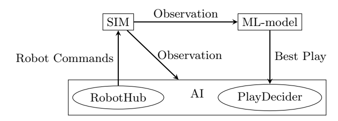
In this context, the proposed simulator is designed to be easily integrated into a gym environment, which allows the use of the Stable Baselines 3 framework to train the model. The trained model will then generate a preferred play as the action space, which is subsequently transmitted to the RoboTeam Twente AI (RTT AI). The RTT AI, in turn, calculates the corresponding robot commands based on the given play. These robot commands are then sent to the simulator, which updates the field and provides observations to the machine learning model. This process is then repeated in an iterative loop, allowing the model to continuously learn and improve its performance. A visual representation of the data flow can be found in Figure 8.

Path Planning Path Planning is a crucial aspect in robot football. Due to the dynamic nature of the environment, generating optimal trajectories that balance time and computational efficiency is imperative. The current strategy employs the use of bang-bang trajectories for time optimisation and implements obstacle avoidance by continuously monitoring the generated path for collisions. In the event of a collision, the trajectory is recalculated with a buffer radius from the detected obstacle, but this results in slower computations and represents a bottleneck in the current AI system.

To enhance the current approach, a novel path planning strategy is proposed. This involves the use of Bezier curves as reference trajectories, which leads to smoother paths that incorporate obstacle avoidance. This is achieved by treating the robots on the field as obstacles and modifying the Bezier curves using rational Bezier curves to avoid sub-optimal paths. The path tracking is managed using a PID controller, which makes adjustments to the heading angle and path deviation through the implementation of piece-wise bang-bang control. This allows the robot to attain maximum velocity along the generated reference path, with necessary corrections made. To prevent collisions with obstacles, a Kalman filter is used for robots in proximity to the path. This allows for a better determination of the feasibility of the generated path and subsequent modification of the rational Bezier ratios if necessary.

The path planning algorithm is based on the work presented in [2]. This algorithm optimises the following constraint:

$$(\dot{X} + \ddot{X})^2 + (\dot{Y} + \ddot{Y})^2 \le 1 \tag{1}$$

Where X and Y are normalised positions in x- and y-direction, respectively. $\dot{X}$ and $\dot{Y}$, and $\ddot{X}$ and $\ddot{Y}$ therefore represent the velocity and acceleration of the robot in x- and y-direction, respectively. The algorithm presents several benefits, including the ability to generate smooth trajectories through the utilisation of Bezier curves. The use of the robot's angle at a specific time step and its corresponding acceleration enables the calculation of updated position and velocity for the next time step.

$$\mathbf{v}_{n+1} = \mathbf{v}_n + h\mathbf{a}_n \tag{2}$$

$$\mathbf{z}_{n+1} = \mathbf{z}_n + h\mathbf{v}_n + \frac{h^2}{2}\mathbf{a}_n \tag{3}$$

where $\mathbf{v}n$ is the velocity at the current time step, $\mathbf{v}{n+1}$ is the velocity at the next time step, h is the sample time, $\mathbf{a}_n$ is the acceleration at the current time step, and $\mathbf{z}_n$ is the position. The $\theta_n$ needed to compute the acceleration can be calculated using two modes: 'Intersect Reference Trajectory' (IR) and 'Out of Reference Trajectory' (OR). The IR trajectory accounts for real noise in the system, which is a feature of this algorithm that allows for better path tracking. IR mode: The IR mode can be computed using

$$\theta_n = \phi + \zeta \tag{4}$$

The Equation (2) and Equation (3) can be rewritten as:

$$\mathbf{c}{n+1} = \begin{bmatrix} x_n \ y_n \end{bmatrix} + \left( h - \frac{h^2}{2} \right) \begin{bmatrix} v{x_n} \ v_{y_n} \end{bmatrix}$$ (5)

$$\mathbf{r}_{n+1} = \frac{h^2}{2} \begin{bmatrix} \cos(\theta_n) \ \sin(\theta_n) \end{bmatrix} \tag{6}$$

Each point on the generated Bezier curve can be represented as $X(\lambda)$ and $Y(\lambda)$. The point closest to $\mathbf{c}{n+1}$ must be calculated. This can be done by first defining a function, which takes the difference between the point on the reference trajectory $(X(\lambda),Y(\lambda))$ and $\mathbf{c}{n+1}$. The argument of the minimum of this function can be found to find the point along the generated curve where the point p is closest to $\mathbf{c}_{n+1}$.

$$f(\lambda) = (X(\lambda) - c_{x_{n+1}})^2 + (Y(\lambda) - c_{y_{n+1}})^2, \quad \lambda \in [0, 1]$$ (7)

$$\lambda^p = \arg\min_{\lambda \in [0,1]} f(\lambda) \tag{8}$$

$$p = P(X(\lambda^p), Y(\lambda^p)) \tag{9}$$

The slope of the tangent can now be used to find $\phi$ and $\zeta$ using:

$$\phi = \tan^{-1} \frac{\dot{Y}(\lambda^p)}{\dot{X}(\lambda^p)} \tag{10}$$

$$\zeta = \sin^{-1}\left(\frac{2|p - \mathbf{c}_{n+1}|}{h^2}\sin(\pi - \gamma + \phi)\right)$$ (11)

where $\zeta$ is the signed angle of the direction of vector $\mathbf{c}_{n+1}$.

OR mode: This mode involves using PID steering control to compensate for the cross track error, $y_{err}$ and the heading error $\psi_{err}$. The cross track error is the distance between p and $\mathbf{c}_{n+1}$ and the heading error is the angle difference between the current heading angle and the slope of the tangent p.

The $\theta_n$ commands can be found using the following PID controllers:

$$\delta \psi = k_p y_{err} + k_d \psi_{err} + k_i \int y_{err} dt$$ (12)

where $\delta \phi$ is the deflection of the heading of the robot, represented by:

$$\delta\psi = \psi_{n+1} - \psi_n \tag{13}$$

and where $\theta_n$ can be found using:

$$\theta_n = \psi_{n+1} + \sin^{-1}\left(\left(\frac{1}{h} - 1\right)|v_n|\sin(\delta\psi)\right)$$ (14)

The papers algorithm also guarantees the optimal condition while satisfying the dynamic constraint within the time interval. This is done by refinement of the acceleration. This is done by:

$$\dot{a}_n = a_1^p + km \tag{15}$$

where $a_1^p$ can be found using:

$$a_n = \frac{2(z_{n+1} - z_n - v_n h)}{h} \tag{16}$$

m is $m = - \left[ \dot{X}(\lambda^p) ; \dot{Y}(\lambda^p) \right]^T$ for the IR mode and is

$$m = -\left[\cos(\psi_n + \delta\psi \sin(\psi_n + \delta\psi)\right]^T$$

k can be found by solving the polynomials of the following equation:

$$ak^2 + bk + c = 0 (17)$$

$$a = (1+h)^2 (m_x^2 + m_y^2) (18)$$

$$b = 2(1+h)\left[m_x(v_{x_n} + (1+h)a_{x_n}^p) + m_y(v_{y_n} + (1+h)a_{y_n}^p)\right]$$ (19)

$$c = ((1+h)a_{x_1}^p + v_{x_n})^2 + ((1+h)a_{y_1}^p + v_{y_n})^2 - 1$$ (20)

Early version UI of the high level simulator.

4.3 Control

This year, the control team was mainly focused on stabilising the already existing control software and improving the control of the dribbler. The improvements made regarding these topics will be elaborated on in this section.

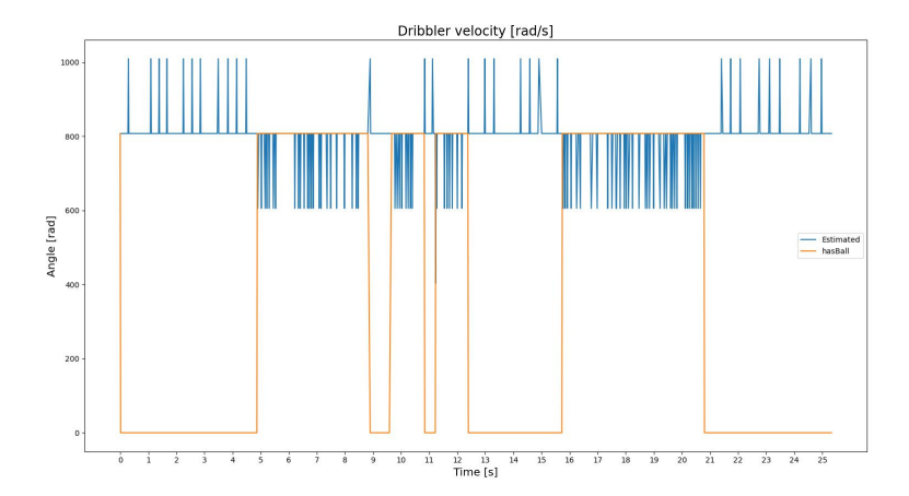
Dribbler as ball sensor Between the last [5] and this ETDP, progress was made in obtaining feedback from the dribbler motor encoder. Connecting the dribbler motors to simple one-pulse encoders did not allow for accurate dribbler control, but turned out to be useful in the form of a rudimentary ball sensor. In addition to the IR-based ball sensors that have been introduced in the TDP from 2018 [3], ball possession can now be determined by observing the rotational dribbler velocity. When this is lower than the rotational dribbler velocity without a ball, it is most likely that the robot is in possession of the ball.. This feature proved to be very useful during the RoboCup 2022.

To fully determine if the ball is in possession, three requirements have to be fulfilled:

1. The rotational dribbler velocity should have reduced compared to the rotational velocity when the robot is not in possession of the ball;
1. The measured rotational dribbler velocity has to be above a given threshold;
1. The dribbler should actively be rotating.

The first requirement assumes that the ball causes friction on the dribbler, making it harder to spin around, causing a reduced rotational velocity of the dribbler bar. The second statement is important for reliability reasons. During testing, as shown in Figure 9, the feedback is not always the most stable. Last but not least, the commanded rotational dribbler velocity should not be zero or decreasing since this would decrease the measured rotational dribbling velocity. The old implementation of this system only checked if there was a rotational velocity commanded to the dribbler, since it used a boolean (full power, or no power). This has been changed as a result of the improved dribbler control that will be discussed in Section 4.3.

To determine if ball possession is lost, two requirements have to be fulfilled:

1. The rotational dribbler velocity should have increased;
1. The rotational dribbler velocity should be very close to the original rotational velocity before ball possession

Once ball possession is lost, the friction that the dribbler motor endures becomes less, allowing it to increase its speed once more with the same amount of energy being fed into it. Since the rotational velocity of the dribbler is not constant, but it tends to jump around a bit, ball possession is deemed to be lost once the speed comes very close to its original velocity, before it obtained ball possession. Of course, another option that allows loss of ball possession is by turning off the dribbler. This bypasses both requirements mentioned above. However, it should be noted that this generally should not happen, since the dribbler is rarely stopped when the ball is in possession. As previously mentioned, individual measurements of the rotational velocity of the dribbler tend to differ. This issue is solved by making use of a moving average, smoothing out the measurements that have been taken. The reason for the difference in individual measurements are mainly that the ball might not constantly be in contact with the dribbler bar, even though the robot does actually have the ball in its possession.

Improved dribbler control Inspired by videos demonstrating the capabilities of ZJUNlict's robots, the aim was to improve the dribbler and hence ball control in the same manner as is described in the ETDP of ZJUNlict [4]. To accomplish this, the chipper was used as a third contact point for the ball, but more importantly, a controller was implemented to influence the rotational dribbler velocities, making it compatible with the angular velocity of the ball.

Measured angular velocity of the dribbler (blue), and the detection of a ball (orange)

References

Brockman, G., Cheung, V., Pettersson, L., Schneider, J., Schulman, J., Tang, J., Zaremba, W.: Openai gym. https://github.com/openai/gym (2016)
Choi, J.w., Curry, R.E., Elkaim, G.H.: Obstacle avoiding real-time trajectory generation and control of omnidirectional vehicles. In: 2009 American Control Conference. pp. 5510–5515 (2009). https://doi.org/10.1109/ACC.2009.5160683
Doornkamp, C., van Egdom, Z., Humblot-Renaux, G., Klute, L., Leunissen, A., Manterola, N., Shipper, S., Sculac, L., Steerneman, E., Tersteeg, S., Vanderwalt, C., van Veelen, W., Wang, H., Weener, J., Jelle, Z.: Roboteam twente 2018 team description paper (2018), https://ssl.robocup.org/wp-content/uploads/2019/01/2018_TDP_RoboTeam_Twente.pdf
Huang, Z., Chen, L., Li, J., Wang, Y., Chen, Z., Wen, L., Gu, J., Hu, P., Xiong, R.: Zjunlict extended team description paper for robocup 2019 (2019). https://doi.org/10.48550/ARXIV.1905.09157, https://arxiv.org/abs/1905.09157
Monat, C., Dankers, E., Skurule, K., Steenmeijer, L., Sijtsma, S., Diamantopoulos, S., Aggarwal, R., Smit, T., van Harten, A.: Roboteam twente extended team description paper for robocup 2022 (2022), https://ssl.robocup.org/wp-content/uploads/2022/04/2022_ETDP_RoboTeam-Twente.pdf
Ommer, N., Ryll, A., Geiger, M.: Tigers mannheim extended team description for robocup 2022 (2022), https://ssl.robocup.org/wp-content/uploads/2022/04/2022_ETDP_TIGERs-Mannheim.pdf
Raffin, A., Hill, A., Gleave, A., Kanervisto, A., Ernestus, M., Dormann, N.: Stablebaselines3: Reliable reinforcement learning implementations. Journal of Machine Learning Research 22(268), 1–8 (2021), http://jmlr.org/papers/v22/20-1364.html
Rahimi, M.M., Segre, J., Monajjemi, V., Koochakzadeh, A., MohaimenianPour, S., Ommer, N., Kimura, A.K., Feltracco, J., Sato, K., Ahsani, A.: Grsim. https://github.com/RoboCup-SSL/grSim/ (2021), gitHub repository
RoboTeam Twente: Roboteam embedded messages. https://github.com/RoboTeamTwente/roboteam_embedded_messages (2023)