TIGERs Mannheim
Michael Ratzel, Mark Geiger, André Ryll
Department of Information Technology Baden-Württemberg Cooperative State University, Coblitzallee 1-9, 68163 Mannheim, Germany
Abstract This paper presents details of the 2D trajectory generation algorithm of the TIGERs Mannheim, a Small Size League (SSL) team intending to participate in RoboCup 2023 in Bordeaux, France. This year, the ETDP will focus on extending the trajectory generation to allow for better goal-shot intercepts of the goalkeeper. The current timeoptimal second-order BangBang trajectories include a complete stop at the intercept destination, wasting valuable time. This is overcome by generating virtual destinations for the robot, that overshoot the intercept point and avoid the preliminary braking, while ensuring the keeper will reach the intercept point at the same time as the ball.
1 Introduction
This paper presents an extension to the current system for generating 2D trajectories that improves the goalkeeper performance when catching shots on the goal. The currently generated second-order trajectories are time-optimal with constant acceleration and include a full stop to reach zero velocity at the specified destination position. However, this full stop wastes valuable time when intercepting goal kicks, and as long as the goalie and the ball are at the interception point at the same time, it is irrelevant that the goalie comes to a full stop at the intersection point in a time-optimal manner.
Since the TIGERs robots are controlled only by specifying the final destination at which the robot should stop, we present an extension algorithm that can provide virtual destination positions such that the actual destination is reached at a given time by an actual trajectory created to the virtual destination. Since this problem is overdetermined, as the robot is not always able to reach the destination in the given time, a best possible virtual position is generated that brings the robot as close as possible to the destination in the given time.
2 Related Work: Untimed Trajectories
The RoboCup Small Size League (SSL) is a fast paced robot soccer league, and due to the high power of the motors compared to size and weight, the omnidirectional drive system of the robots is mainly limited by friction. Therefore, the Cornell Big Red team has presented an approach that generates secondorder time-optimal trajectories with constant acceleration and a complete stop at a given target destination [1]. The current implementation is based on this approach and is discussed in more detail in section 3.
The work of Hove et al. [2] presents a problem similar to intercepting a goal shot: Catching a ball with a robotic arm. However, they must impose more stringent requirements on the trajectory of the arm's end effector as they attempt to match the position, velocity, and acceleration of the ball at the interception point to reduce the risk of the ball bouncing off the arm. For future offensive applications, such as receiving a pass with a moving robot, these requirements may also be imposed, but for simply intercepting a shot on the goal, whether the ball bounces off the goalkeeper is irrelevant, and trying to match velocity and acceleration wastes valuable interception time.
In the "Mousebuster" work, an attempt is made to catch a mouse with a robotic arm. Here, the end effector of the robot does not have to match the velocity of the mouse, so the problem is closer; instead, an attempt is made to catch the mouse by placing a cup over it on the floor. Therefore, the velocity of the robot at the point of contact must be 0 to avoid hitting the ground. As mentioned earlier, this full stop again wastes valuable time. Furthermore, the trajectory presented in the paper is a third-order jerk-limited trajectory. The TIGERs use only second-order acceleration-limited trajectories because the robots are built to withstand very high jerks in collisions with other robots, and the motors are powerful enough to generate the large acceleration jumps. More details on the TIGERs robots can be found in the team's latest publications [3–5].
3 Current Approach: Untimed Trajectories
As mentioned earlier, our current approach for time-optimal 2D BangBang trajectories is based on the approach presented by Cornell Big Red [6, 1]. It consists of two 1D trajectories for the two orthogonal axes $x$ and $y$ in the plane of the field. Each 1D trajectory consists of up to 3 phases with constant acceleration. An acceleration phase, an optional plateau phase with maximum velocity and an second acceleration phase. Each phase is described by the following equations of motion, with the position $s(t)$, the initial position of the phase $s_0$, the velocity $v(t)$, the initial velocity of the phase $v^0$ and the constant acceleration $a$ is either zero or the positive or negative limit $\pm a_{\text{max}}$ .
$$s(t) = s_0 + v_0 t + \frac{1}{2}at^2$$
$$v(t) = v_0 + at$$
$$a = \text{const}$$
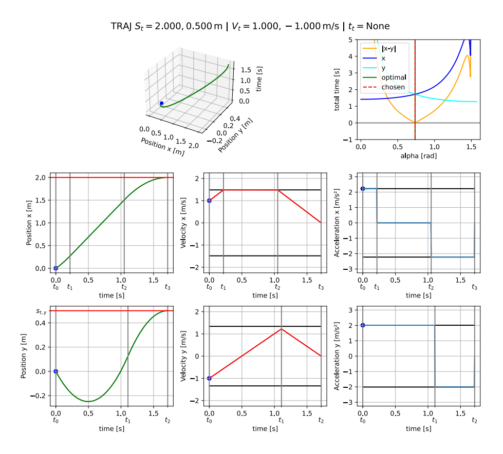
A 2D trajectory is shown in fig. 1 that starts at $S_0 = (0,\mathrm{m}, 0,\mathrm{m})^T$ with an initial velocity of $V_0 = (0,\mathrm{m,s^{-1}}, 1,\mathrm{m,s^{-1}})^T$ , ends at the given destination $S_t = (1.5,\mathrm{m}, 0.5,\mathrm{m})^T$ , and has a maximum velocity of $v_{\mathrm{max}} = 2,\mathrm{m,s^{-1}}$ and a maximum acceleration of $a_{\mathrm{max}} = 3,\mathrm{m,s^{-2}}$ . The bottom two rows of the figure show the position, velocity, and acceleration of the 1D trajectories of the x and y axes, with the target destination marked as a horizontal red line in the position graph. The 1D graphs have marked time stamps: the transition times of the phases $t_0, t_1, t_2[, t_3]$ . These are used in the following to assign variables to specific time points or time intervals. A position, velocity, or acceleration with a single index specifies its value at the exact time stamp, e.g., $s_i = s(t_i)$ is the position exactly at $t_i$ . Variables with two indices describe the difference, e.g., $s_{i,j} = s(t_j) - s(t_i)$ , or $t_{i,j} = t_j - t_i$ .
The velocity profile of the x-axis in the middle clearly shows all three possible phases: $t_{0,1}$ the acceleration phase one, $t_{1,2}$ constant velocity phase and $t_{2,3}$ acceleration phase two. Overall, the velocity resembles a trapezoidal shape. The y axis has only the two acceleration phases $t_{0,1}$ and $t_{1,2}$ , which resembles a triangular velocity shape. The constant velocity phase is omitted for the triangular shape because the distance on the y-axis is not long enough to accelerate to $v_{\rm max}$ and decelerate back to 0.
In order to enforce the maximum velocity and acceleration that the robot's hardware can achieve, we need to solve the optimization problem of what fraction of the total maximum velocity and acceleration can be assigned to each 1D trajectory. We can formulate the problem as finding the optimal angle $\alpha$ and computing from it the respective velocity and acceleration maxima using the following equations:
$$v_{\max,x} = v_{\max} \cos \alpha$$
$$a_{\max,x} = a_{\max} \cos \alpha$$
$$v_{\max,y} = v_{\max} \sin \alpha$$
$$a_{\max,y} = a_{\max} \sin \alpha$$
The maxima are used to compute the total time $t_{\rm total}$ of the 1D trajectories. In the upper right corner of fig. 1 we see the total times of the x (dark blue) and y (light blue) trajectories in relation to $\alpha$ , and the absolute difference between these times in orange. For a time-optimal 2D trajectory, the difference must be 0. This is indicated by the green vertical line. The dashed red line marks the $\alpha^*$ chosen by the implemented optimization strategy. Since the absolute time difference is mostly convex (see section 5.2), we use a binary search approach.
4 Overshooting Trajectories
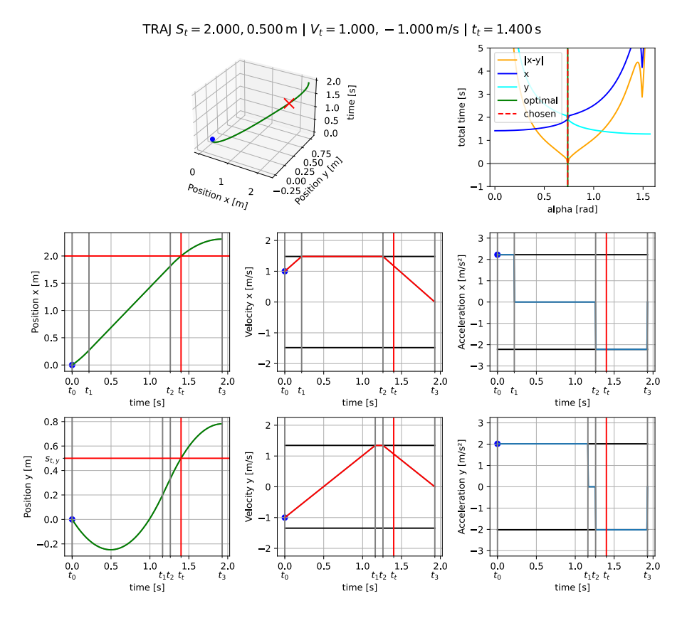
The extension now adds an extra input for the trajectories, not only the 2D destination $S_t$ , but also a wanted arrival time, the target time $t_t$ is given. It is marked in the 1D graphs as a vertical red line, while the 2D graph marks only the timed target position $(s_{t,x}, s_{t,y}, t_t)^T$ with a red cross, as shown in fig. 2.
The new output of the extension are virtual destinations $S_t^$ , so $s_3$ of the x and y graphs in fig. 2. This virtual position $S_t^ = (s_{3,x}, s_{3,y})^T = (s_{t,x}^, s_{t,y}^)^T$ is then sent to the robot as a normal target destination, and the robot will drive there with a trajectory generated by the current approach, as the virtual position is created such that the robot passes the target destination at the target time. The virtual destinations can be placed behind the actual destination $S_t$ to avoid the unnecessary breaking before reaching $S_t$ , or exactly at $S_t$ if $t_t$ is large enough to allow for a full stop. We call trajectories where the robot drives further than the actually wanted destination overshooting trajectories, and they can be either a forced overshoot: The robot is too fast and passes the destination before the target time, so it overshoots and has to recover. Or they can overshoot deliberately, so that the robot heads for a virtual destination in order to reach the actual destination just in time.
For the generation of 2D virtual positions, the extension reuses the same $\alpha$ optimization strategy used in the existing approach, but replaces how 1D trajectories are generated. The new 1D trajectories to the virtual destination are generated, such that they get as close as possible to the target destination at the target time point. The total time $t_{\text{total}}^$ and final virtual position $s_t^$ of the trajectory are then used in the $\alpha$ optimization generation to combine two 1D trajectories to one 2D one. If the approach is successful and $t_t$ is high enough to allow the robot to hit the target destination in time, the 1D position graph will intersect with both the target time $t_t$ and the target position $s_t$ at the same point, and the 2D position graph intersects the red cross.
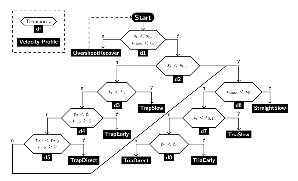
A decision tree summarizing the proposed 1D algorithm is shown in fig. 3. For simplicity, the only case shown is a 1D trajectory from $s_0 = 0$ to $s_t \ge 0$ , since all other cases can be constructed simply by offsetting $s_t$ with $-s_0$ , or multiplying $s_t$ by -1. The eight decisions d1 to d8, as well as the eight resulting velocity profiles, are shown in detail below.
4.1 d1: Forced Overshoot and Recovery Handling
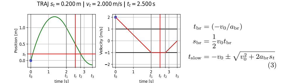
As mentioned at the beginning of the section, not all overshoots are desirable. If the robot is already close to the intercept point and has a high velocity, it is possible that it is too fast to slow down to zero at the final position and overshoots. This is the case when $s_t < s_{\rm br}$ , with $s_{\rm br}$ being the closest position where the robot could fully break, by decelarting the whole way. If the slowest possible time $t_{\rm slow}$ to reach $s_t$ is smaller than $t_t$ , the robot will not only overshoot, but will also be at the intercept point faster than desired despite breaking for the whole distance $s_t$ , as shown in fig. 4.
Setting $s_0^* = s_{\rm br}$ , $v_0^* = 0$ , $t_t^* = t_t - t_{\rm br}$ adjusts the problem to start at $s_{\rm br}$ (at roughly 1.3 s in fig. 4) and focus on recovery after the overshoot. Thus, the robot is no longer too fast, but focuses on being fast enough during recovery, which is the same problem as being fast enough when no overshoot and therfore no recovery is enforced, resulting in one of the seven other velocity profiles plus the preceeding braking phase.
4.2 d2: Trapezoidal Shape Possible
$$a_{0} = \begin{cases} +a_{\text{max}} & \text{if } v_{0} \leq v_{\text{max}} \ -a_{\text{max}} & \text{else} \end{cases}$$
$$t_{0,1} = \frac{v_{\text{max}} - v_{0}}{a_{0}}$$
$$s_{0,1} = \frac{v_{\text{max}} + v_{0}}{2} t_{0,1}$$
The next general decision is whether a trapezoidal velocity provile is possible at all. This is done by calculating the distance $s_{0,1}$ that the robot must accelerate to $v_{\text{max}}$ . If the robot reaches $s_{0,1}$ first $(s_t > s_{0,1})$ , trapezoidal shapes are generally possible and must be checked. If not, the algorithm can proceed directly with d6.
4.3 d3: Trapezoidal Too Slow
$$t_{1,2} = \frac{s_t - s_{0,1}}{v_{\text{max}}}$$
$$t_2 = t_{0,1} + t_{1,2}$$
The first velocity profile checked is acceleration to $v_{\rm max}$ and maintaining that velocity until $s_t$ is reached. With $t_2$ , the total time to reach $s_t$ , we can check if $t_2 > t_t$ . If it is, the robot cannot reach the destination in time without violating $v_{\rm max}$ . The third phase, the braking phase $t_{2,3}$ is added after the destination is reached, and the total time $t_{\rm total}^$ and the virtual destination position $s_t^$ are calculated using eq. (6), resulting in the trajectory shown in fig. 5.

4.4 d4: Trapezoidal Finishing Early
The decisions d2 and d3 imply that a trapezoidal shape is possible in general and it is fast enough to reach the destination before or at tt, the next step is to check if a trapezoidal shape with a full stop is possible so that the trajectory looks as if no t^t is given. To do this, two conditions must be satisfied t1,2 ≥ 0 and t^t > t3, where t0,1 and t2,3 are from eqs. (4) and (6):
$$s_{1,2} = s_t - s_{0,1} - s_{2,3}$$
$$t_{1,2} = \frac{s_{1,2}}{v_{\text{max}}}$$
$$t_3 = t_{0,1} + t_{1,2} + t_{2,3}$$
With an unchanged destination position and t^3 as total time, the trajectory shown in fig. 6 can be created:
4.5 d5: Trapezoidal Direct Hit
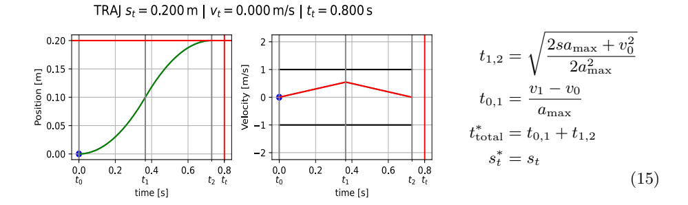
The third trapezoidal form is a direct hit, where the robot will reach the target destination exactly at the wanted time tt, while driving. With s0,1 and t1,0 from eq. (4) the time of the constant velocity phase t1,2 can be calculated with the following equations:
$$s_{1,t} = s_t - s_{0,1}$$
$$t_{1,2} + t_{2,t} = t_t - t_{0,1}$$
$$s_{1,t} = v_{\max} t_{1,2} + v_{\max} t_{2,t} + \frac{1}{2} (-a_{\max}) t_{2,t}^2$$
$$t_{2,t} = \sqrt{\frac{2(s_{1,t} - t_{1,t} * v_{\max})}{-a_{\max}}}$$
$$t_{1,2} = t_{1,t} - t_{2,t}$$
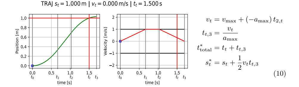
If t1,2 > 0 and t2,3 > t2,t with t2,3 from eq. (6) is true, a direct hit is possible. This results in the following calculation for the final trajectory:
4.6 d6: Straight Too Slow
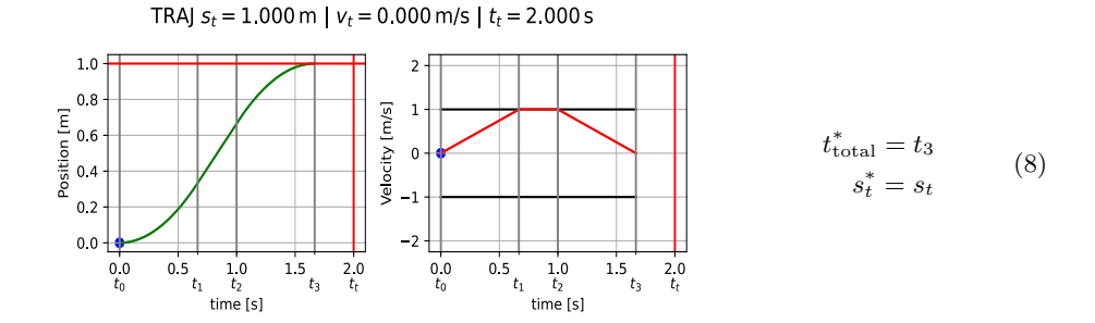
When this point is reached, a trapezoidal shape is no longer possible and a boundary case must occur before the algorithm can proceed with triangular shapes, this is the Straight Too Slow case. If v^0 > vmax and the destination position s^t is reached before the robot could decelerate to v = vmax, it makes most sense to decelerate in a straight line to v = 0 and end the trajectory at this point, as the robot can't be early, as this is handled by the overshoot and recovery detection. The final destination s ∗ t for the trajectory shown in fig. 8 is calculated using the following equations:
Deciding if this shape shall be used is based only on v^0 > vmax, as any other case, with an initial velocity higher than the maximal velocity, is handled by the trapezoidal shapes or forced overshoot and recovery.
4.7 d7: Triangular Too Slow
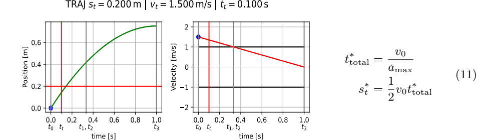
Analogous to the trapezoidal shapes, the triangular shapes will be handled, first check if too slow, then if an early end is possible, and then a direct hit. There are only two reasons why the previous could not find a solution: Either the robot cannot accelerate to vmax before reaching st, or all trapezoidal shapes are too fast at the destination position. So checking for triangular shapes that are too slow only checks if accelerating until reaching the destination is too slow:
$$s_{0,1} = s = v_0 t_{0,1} + \frac{1}{2} a_{\text{max}} t_{0,1}^2$$
$$t_{0,1} = \begin{cases} \frac{-\sqrt{2a_{\text{max}} s + v_0^2 - v_0}}{a_{\text{max}}} & \text{if } s \ge 0\ \frac{\sqrt{2a_{\text{max}} s + v_0^2 - v_0}}{a_{\text{max}}} & \text{else} \end{cases}$$
If t0,1 ≥ t^t triangular is too slow, and the trajectory shown in fig. 9 is generated with the following equations:
4.8 d8.1: Triangular Finishing Early
To decide whether the triangle shape can end prematurely with a full stop, the trajectory is modeled in the same way as for a triangle shape without timing:
$$s_{t} = v_{0}t_{0,1} + \frac{1}{2}a_{\max}t_{0,1}^{2} + v_{1}t_{1,2} + \frac{1}{2}(-a_{\max})t_{1,2}^{2}$$
$$v_{1} = a_{\max}t_{1,2}$$
$$v_{1} = v_{0} + a_{\max}t_{0,1}$$
With this, the $t_{\text{total}}^$ can be calculated, which decides if the triangular finishing early can be used: $t_{\text{total}}^ < t_t$ .
4.9 d8.2: Triangular Direct Hit
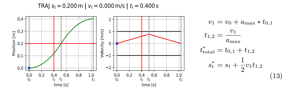
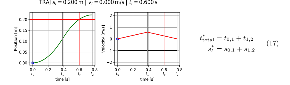
The only velocity profile left is the triangular direct hit, therefore no additional checks are necessary, and the trajectory can be modeled with the following equation:
$$s_{t} = v_{0}t_{0,1} + \frac{1}{2}a_{\max}t_{0,1}^{2} + v_{1}t_{1,t} + \frac{1}{2}\left(-a_{\max}\right)t_{1,t}^{2}$$
$$t_{t} = t_{0,1} + t_{1,t}$$
$$v_{1} = v_{0} + a_{\max}t_{0,1}$$
$$t_{1,t} = \sqrt{\frac{a_{\max}t_{t}^{2} - 2s_{t} + 2v_{0}t_{t}}{2a_{\max}}}$$
$$t_{0,1} = t_{t} - t_{1,t}$$
$$t_{1,2} = \frac{v_{1}}{a_{\max}}$$
$$s_{0,1} = \frac{v_{0} + v_{1}}{2}t_{0,1}$$
$$s_{1,2} = \frac{v_{1}}{2}t_{1,2}$$
Which resolve to the following solution, with fig. 11 as an example:
5 Comparison to Untimed Trajectories
5.1 Increase of the Effective Keeper Range
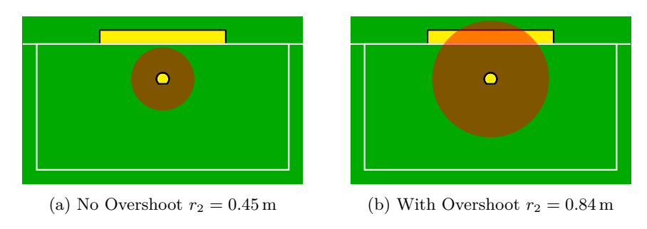
To compare the effect of the overshoot, the situation of a goal shot with 6.5 m s^−1 and a distance of 4 m is constructed. Resulting in travel times for the ball of roughly 0.75 s depending on the carpet and ball model. The distances the keeper can travel within those 0.75 s are drawn around a keeper in front of a Division A goal in fig. 12. Within the 0.75 s the keeper travels without overshooting 0.452 m and with 0.835 m, such that the keeper with overshooting can block all goal shots, that are further away than 4 m. The keeper without overshooting will need 1.055 s to reach the same distance of 0.835 m as the overshooting keeper, which translates to a kick distance of roughly 5.3 m. As mentioned above, these numbers are certainly not completely accurate, as they vary depending on the carpet and also goal shots cannot be detected immediately by the image processing system, but as a rough estimate, over-shooting significantly improves the performance of the goalkeeper.
5.2 Discussion of Non-Convex Alpha Optimization
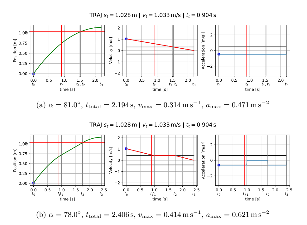
As already mentioned, to find the optimal α we use a binary search like approach, that is based on the assumption, the larger vmax and amax are, the faster a trajectory must finish, as this implies a convex shape for the absolute difference between the two axis times ttotal,x and ttotal,y over the optimization range. As increasing α, increases vmax,y and amax,a, while decreasing vmax,x and vmax,x, and vice versa. Applying the assumption, increasing α increases ttotal,x and decreases ttotal,y and vice versa. So the further away from the optimal point, where ttotal,x = ttotal,y, the bigger the absolute difference |ttotal,x − ttotal,y| will be. But the assumption, the bigger vmax and amax is, the faster the trajectory does not hold for every case. Both for the trajectories with and without overshooting counter examples can be found, of which one is shown in fig. 13. The trajectory in fig. 13a with lower maxima finishes over 0.2 s faster than the one in fig. 13b. Those counterexamples are only possible, if the initial velocity v^0 is greater than vmax, as this anomaly is caused by smaller acceleration amax, causing the trajectory to stay above vmax for a longer time, leading to a faster time in total. If v^0 is below vmax, the assumption always holds, as this was proven in [6].
This problem is the same for timed and untimed trajectories. The α graph in the upper right corner of fig. 1 clearly shows the existence of the problem for untimed trajectories. And these trajectories have been used successfully in the TIGERs software for many years without causing any problems, since this behavior is only noticeable for small α ranges, and only for rather extreme values for α. Also, the anomaly only causes issues, if the normally higher time of one axis drops below the other time, so if the two blue lines would intersect in the α graphs, which is very unlikely. Moreover, the trajectories are updated many times per second with new measurements from the global vision system and the robot's odometry system, so rare cases of incorrectly optimized α values have a negligible impact on overall performance. This disadvantages are outweighed by the high computational efficiency of the binary search approach used.
6 Optimal Ball Interception Point Selection
The selection of the optimal ball interception point is not trivial, the simplest estimate with the foot of the perpendicular of the robot's position and the ball flight line can be improved. If the goalkeeper is standing still and the interception point is moved slightly towards the goal, the distance the goalkeeper has to travel increases only slightly, while the distance the ball travels increases significantly. Knowing how fast the ball and the robot will be at the interception point, it is possible to calculate how far the interception point should be optimally shifted towards the goal. However, the TIGERs keeper rarely stands still during a match and constantly updates its blocking position. Therefore, the calculation becomes more complex as the initial velocity of the robot strongly influences the optimal interception point. We decided to use a sampling approach because the entire trajectory generation process is very performant and can be executed many thousands of times per second. Every ten millimeters along the ball flight line and within the penalty area, a position is sampled. At each position the time it takes for the ball to reach the position is calculated and with this information a trajectory to a virtual destination is generated.
Trajectories are then selected via the following criteria: distance to the intersection point, velocity, distance to the goal line, and finally time remaining. Thus, if the goalkeeper cannot reach the destination within the remaining time at any interception point, the trajectory with the smallest distance to the ball at its intersection time is selected. If there are multiple locations where the ball can be reached, the one where the goalie is slowest is selected, as this increases both accuracy and the margin for adjustments to the destination in the next frame. If there are multiple positions where the goalie can come to a stop in time, we prefer positions farther from the goal line. However, only within the first 0.27 m (3 bot radii), since we consider any interception point further away to be safe. If there are multiple positions where the ball can be intercepted with a full stop that are further than 0.27 m from the goal line, the final decision criterion is to maximize the time between the goalkeeper's arrival and the ball to maximize the margin for future adjustments.
7 Conclusion
This paper describes an extension to the existing system for generating 2D trajectories. Unlike the existing approach, this extension does not guarantee that the robot will reach a destination point in an optimal time manner, including a full stop. This additional freedom allows the robot to reach the actual destination faster by removing the full stop constraint, while the extended algorithm ensures that the robot reaches the destination at a desired time, such as when intercepting a goal kick.
Since our goalkeeper only had to intercept two goal shots during the entire 2022 RoboCup tournament, and neither shot required an overshot, we cannot support the claims in this paper with real tournament data. However, field tests in our laboratory have shown that the claim made in section 5 that the goalkeeper's effective range was nearly doubled is reasonable.
References
- Purwin, O., D'Andrea, R.: Trajectory generation and control for four wheeled omnidirectional vehicles. Robotics and Autonomous Systems 54(1), 13 – 22 (2006). https://doi.org/10.1016/j.robot.2005.10.002
- Hove, B., Slotine, J.J.E.: Experiments in robotic catching. In: 1991 American Control Conference. pp. 380–386 (1991). https://doi.org/10.23919/ACC.1991.4791395
- Ommer, N., Ryll, A., Geiger, M.: TIGERs Mannheim Extended Team Description for RoboCup 2022 (2022)
- Ryll, A., Jut, S.: TIGERs Mannheim Extended Team Description for RoboCup 2020 (2020)
- Ryll, A., Ommer, N., Geiger, M.: RoboCup 2021 SSL Champion TIGERs Mannheim - Ball-Centric Dynamic Pass-and-Score Patterns. In: Alami, R., Biswas, J., Cakmak, M., Obst, O. (eds.) RoboCup 2021: Robot World Cup XXIV. pp. 241–257. Springer International Publishing (2022)
- Kalmar-Nagy, T., D'Andrea, R., Ganguly, P.: Near-optimal dynamic trajectory generation and control of an omnidirectional vehicle. Robotics and Autonomous Systems 46(1), 47–64 (2004)