ER-Force 2024 Extended Team Description Paper

Theodor Böhm, Elisabeth Gareis, Undine Hahn, Tobias Heineken, Valentin Hopf, Michel Schmid, Christoph Schmidtmeier, Marco Wiedmann

Friedrich-Alexander-Universität Erlangen-Nürnberg (FAU), Faculty of Engineering, Department of Computer Science, Distributed Systems and Operating Systems Robotics Erlangen e.V., Martensstr. 1, 91058 Erlangen, Germany

https://www.robotics-erlangen.de/

Abstract This paper presents the proceedings of ER-Force, the RoboCup Small Size League team from Erlangen located at Friedrich-Alexander-University Erlangen-Nürnberg, Germany. It describes the manufacturing process of our robot covers, as well as electronic simulations and measurements of our kicking assembly. Furthermore, it explains the statistical methods we use in our strategy to make it robust against noise in the vision data.

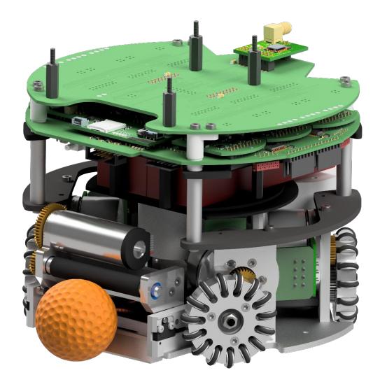
Figure 1: ER-Force robot design from 2023

[No text in abstract]

1 Introduction

This ETDP presents our recent improvements to the mechanics, electronics and AI. Section 2 explains and compares our robot cover production process to other alternatives. Subsequently, section 3 develops a simple electrical model for the electronic part of our kicker. Finally, section 4 explores various methods to deal with noisy data in the AI with detailed examples.

2 Mechanics - Robot Cover

The outermost part of a robot is its cover. It protects the inside during crashes, thus it is objected to wearout. With this in mind and eventual changes in size of new robot generations we need new covers from time to time. We use a low cost and easy to manufacture design, which is adaptable to different robots. In the following section we will explain the production of our cover first and give a conclusive overview to its specific advantages and disadvantages.

2.1 Production Process

Our cover is mainly built from 1 mm thick polystyrene. Hot glue is used to assemble the pieces. Additionally, some tools are needed: a laser cutter, an iron pipe with approx. diameter and height of the robot, a pot with a fitting lid, a (portable) stove top, some magnets and some heat protective gloves. The pot needs to be big enough to fit the iron pipe - standing up - into it.

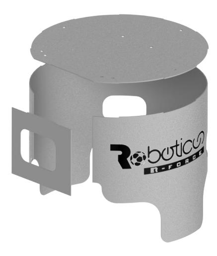
Our robot cover consist of three different parts as seen in fig. 2, which are cut out of a polystyrene sheet using a laser cutter. The flattened view is cut out for the bent side part. An additional fourth part is used for the vision pattern and thus consists of a black material. This resembles the top part, but with cut-outs for the pattern circles.

After all parts are cut, the flat side part must be brought into its circular shape. As polystyrene is a thermosoft plastic, it can be easily deformed at a sufficiently high temperature and keeps the shape after cooling back down. A pot in combination with a piece of an iron pipe is used to deform the material. The pot is filled with a small amount of water. As the hot steam is sufficient to heat the polystyrene, the water should not directly touch the polystyrene once the core is inserted into the pot.

Polystyrene may emit toxic fumes during the heating process. For this reason we suggest using a portable stove top in the open air and masks.

Before putting the pipe in the pot, the side part is placed inside it and fixed using magnets. Once the water starts to boil the core can be inserted into the pot and lid put on top. The time needed to cook the polystyrene is influenced by the temperature, the amount of water and the material used. After getting the timing by trial and error, the process is reproducible. The polystyrene is finished just before the pattern edges start to form waves. Once the cover side is deemed fully cooked, the core is removed from the pot with the help of heat protective gloves and the magnets can be removed. The cover should now retain its shape, which corresponds to the diameter of the robot. If not, the sheet can be put back inside the core and it can be cooked a bit longer.

As a last step the cover parts are connected to each other. Experience has shown that the cover should be assembled with the help of masking tape first, as it is quite difficult to connect the bent side panel. This helps improve the alignment seen in fig. 3 and fit of the different cover pieces and simplifies assembly. The small cogs visible in fig. 3 additionally support the precise assembly. Next hot glue is spread on the inside seam of the cover to fuse the pieces together.

The pink and green paper cut-outs for the robot number are glued to the bottom side of the pattern plate and thus do not need to be cut out exactly.

Plastic screws and nuts connect the pattern plate to the top part of the cover. As a final step the team color is slid in from the front between top and pattern plate. A 3D model of our cover and the part files can be found in our 2023 open source publication.[1]

2.2 Comparison

After introducing the manufacturing process, we want to highlight some aspects of our cover and why we think it may be suitable for some other teams as well.

• Tools: The majority of tools used to produce our covers is standard household equipment, which can be bought from a hardware store for relatively cheap everywhere. The only special equipment needed is a laser cutter, but many places offer cutting as a service. We do not own a laser cutter by ourselves as well.
• Production time: Compared to a 3D printed cover as in [1] and [2] which may take several hours to print per piece, our manufacturing process is quite fast. All covers for 16 Robots were produced in approximately 6 hours.
• Price: Apart from that, the long 3D printer occupancy for covers leads to a high cost. The manufacturing of our cover costs approximately 6 e per piece. It is therefore a good solution for teams with less financial capabilities.
• Mounting: Two pins punching through the covers top plate and relative tight fit of cover to the inner structure of robot is all holding our cover in place. It can be simply slid over the robot. In comparison to brackets [3] or screws [2] this allows for a faster removal of our cover.
• Adaptability: As our cover has very few interfaces to the robot, there is a high chance it will fit a robot not prepared for this type of cover.
• Flat outer surface: As a last aspect we want to highlight the flat outer surface of our cover. This is ideal for applying stickers, for example with a special robot design or sponsorship logos.

In summary cooking the robot covers is an easy, low budget and low time investment approach which can be used by almost anybody. While the cover provides stability and protection it is also easy to apply or adapt.

3 A simple electrical model for the kicker

We are on an ongoing path to optimize the kick of our robot compared to the previous generation. After improving the safety and reliability of the kick in the last paper [4], we now want to improve the efficiency of the solenoid driven by the kicker. The objective is to optimize the velocity of the solenoid plunger while minimizing the thermal losses in the solenoid coil.

The goal of this section is to determine the efficiency of the current kicker. The mechanical and electrical design is open-source[2] .

Since we use no internal current sensing like for example hall sensors [5], a LTspice simulation is used to estimate the currents and voltages occurring during the discharge process. This is necessary to determine the required measurement configuration in order to avoid damaging the equipment.

We validate the simulation with measurement data and use it to determine the outgoing velocity of the ball and thermal losses.

3.1 Simulation in LTSpice

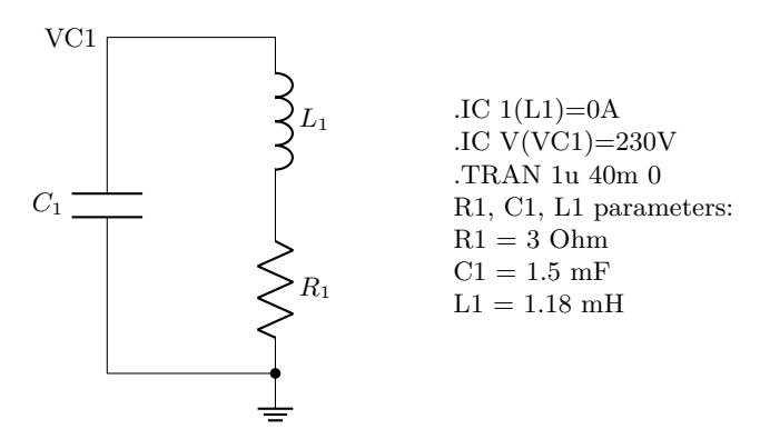
For the simulation in LTspice we use a simplified model of the circuit (confer fig. 4). Using a more complicated model would require a simulation of the fields inside the coil [6]. We assume an ideal capacitor with no parasitic inductance or resistance. The Resistance and inductance of the solenoid coil are orders of magnitude bigger and outweigh the parasitic effects. The inductance of the coil was measured at 1.18 mH. The capacitance of the kick circuit is 1.5 mF. The ESR (equivalent series resistance) of the capacitors is in the range of tens of mΩ while the resistance of the coil is 3 Ω, therefore we can ignore the ESR of the capacitor. The same logic applies to the parasitic series inductance of the capacitor. Although the manufacturer does not specify this value, the inductance of the solenoid coil is much bigger than the parasitic inductance of the capacitor.

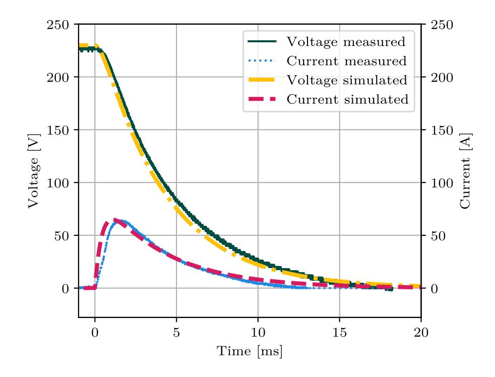
The simulation is a transient analysis of the circuit with initial conditions that represent the instant the discharge begins. The voltage of the capacitor is set to the charge target voltage of 230 V. To simulate the activation of the kick the circuit is already connected to L1 and R1, but the current through these components is set to 0 A. At the start of the simulation the current starts flowing through the closed circuit. The voltage curve (fig. 6, "yellow dash-dotted line") is similar to the theoretical curve of capacitor discharging through a resistor. The current curve (fig. 6, "purple dashed line") peaks around 65 A which poses a challenge to measure in the lab.

3.2 Measuring the current and voltage

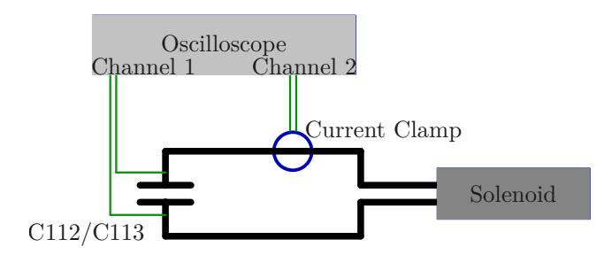
An oscilloscope with a 1:10 probe on Channel 1 was used to measure the voltage of the coil (fig. 5) by probing at the pins of the capacitors. Directly measuring the current with an inline amperemeter was not an option, because of the predicted current peak around 65 A and most amperemeters have a maximum range of 10 amps. The other option we considered was using a current shunt resistor but because the resistance of the coil is so small adding a resistor could change the system itself and taint the measurement. The solution we settled on is using a current clamp with a sufficient range on Channel 2 (fig. 5).

The data was captured in single-shot mode. The trigger was set on Channel 1 (the capacitor voltage) and slightly below 230 V, because 230 V is the voltage of the capacitors before the discharge begins.

3.3 Comparing the results

The results of the measurement can be seen in fig. 6 as the black and blue lines. The LTspice simulation was able to make a good estimate of the currents and voltages. An obvious issue with LTspice is that the simulation conserves the energy of the system and therefore all energy in the capacitors will be turned into heat losses at the resistor. There is no component in the simulation to account for the energy transferred to the ball. Another source of inaccuracy is the inductance of the coil. The value used for the simulation assumes a constant value but in reality the inductance is dependent on the position of the plunger within the coil. The total theoretical energy $E^t$ available in the capacitors is dependent on the voltage and size of the capacitor:

$$E_t = \frac{1}{2}V^2C = 39.675 ,\mathrm{J} \tag{1}$$

The total real energy $E^m$ converted form the capacitors can be calculated by integration of the power $P$ = $UI$. This is done using numerical integration with Riemann sums and the samples of measurement.

$$E_m = \int_{t=0 \text{ ms}}^{20 \text{ ms}} U_m(t) I_m(t) dt = 38.4 \text{ J}$$ (2)

This shows an inaccuracy of the simulation to the real world of 3.4% regarding the total energy of the discharge. The energy lost at the resistance of the coil $E_{dm}$ in the measurements can also be calculated with eq. (3).

$$E_{dm} = \int_{t=0 \text{ ms}}^{20 \text{ ms}} I_m(t)^2 R_{coil} dt = 36.5 \text{ J}$$ (3)

The remaining Energy is transferred into the plunger and therefore into the ball $E_b$:

$$E_b = E_m - E_{dm} = 1.78 ,\text{J} \tag{4}$$

The efficiency $\eta$ of the kick is:

$$\eta = \frac{E_b}{E_m} = 4.6% \tag{5}$$

While the measured efficiency of our kicker at less than 5% is not great, transferring 1.78 J to the ball is theoretically enough to accelerate the ball to 9.1 m s limit of 6.5 m s . Therefore, this two-step approach of simulation followed by measurements shows our current kicker to transfer enough energy.

4 Using statistics in the AI: best practices and examples

Any SSL team has to deal with the fact that all information they have about the situation on the field is fundamentally inexact. In particular, the data supplied by the vision system is inherently noisy. While a custom tracking system can somewhat compensate for this [7, 8, 9, 4, 10, 11], it will never be perfect. For example, seemingly simple questions like "is the ball currently moving" already require some heuristics on the estimated ball position and speed, since the latter will for all practical purposes never be exactly zero.

Statistics provides us with some useful tools to deal with noisy data. While even the most advanced statistical methods will not be able to eliminate all uncertainties, they can at least help to further improve the reliability of the resulting metrics. Since the problem of noisy data is so generic that we are confident that every team should apply statistics to the field state, we want to share some best practices and provide concrete examples on what can be achieved.

4.1 Motivation

[Included in section 4 introduction]

4.2 Using ring buffers to store data

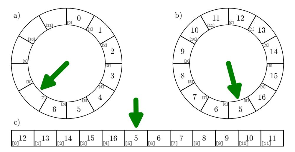
For many statistical methods, multiple measurements of the quantity in question need to be gathered and stored. Commonly one wants to look at the last $n$ samples of this quantity to evaluate some metric. Examples include calculating the mean of the past ball positions or correlations in the ball's movement direction. Ring buffers provide an elegant way of managing a constant number of past observations (see fig. 7). Each time a data point is stored in the buffer, the oldest entry is automatically overwritten with the new one. This ensures that one always works with the most recent data.

The correct length of the buffer depends on the specific problem at hand. Including more samples leads to robuster results but comes at the cost of a more inert metric. As SSL games are in their very nature dynamic situations, the state of the field will change, sometimes very rapidly so. Whatever metric or criterion one is trying to build needs to be able to pick up on these changes quickly so the AI has enough time to react. Since there is no general best solution, we try out different buffer sizes and see if the results are stable enough and still react to changes in time.

Some care needs to be taken with freshly initialized buffers. Since they are not yet completely filled with actual measurement data, metrics calculated on the buffer might be wildly inaccurate on the first few iterations. In these cases the developer can either choose to only include the available data, risking that the resulting metric might fluctuate a lot in the beginning. Or one can fall back to some default assumption on the field state, which is at least stable but might be flat out wrong.

Another situation which needs to be handled more carefully arises when data becomes obsolete, but new data might not already be available. For instance one might only consider the ball detections from the past second. Since sometimes the ball is not visible at all, it is not possible to ensure that obsolete detections are overwritten in the ringbuffer immediately.

4.3 Applying hysteresis on discrete decisions

Hysteresis is a technique to avoid rapid switching between discrete outcomes whenever a noisy, continuous variable is used for the decision process. While it is wide-spread among SSL teams [11, 12, 13, 14] and has briefly been covered in [15], it is an important enough concept to deserve a more detailed explanation.

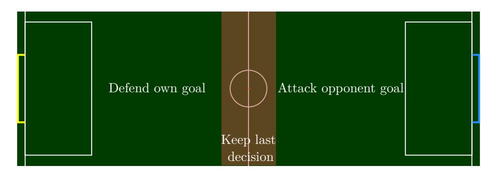
As an instructive example, consider the following situation. A very simplistic SSL AI might decide whether its robots should be attacking or defending by checking in which half the ball is currently positioned. At the start of the game the ball will be positioned more or less exactly on the halfway line. Therefore, just by the inherent tracking uncertainty the ball will sometimes be detected in one half and sometimes in the other half. Consequently, the decision of the AI will rapidly oscillate between attacking and defending, leaving the robots not enough time to do either.

A hysteresis addresses this problem by defining a region around the decision boundary where the previous decision is always being repeated. In other words: the decision border must be surpassed by some minimal amount in order to trigger a change of behavior. In the example above this means defining an area around the halfway line in which the AI holds onto the decision of the previous iteration (see fig. 8).

This concept can straightforwardly be generalized to multiple possible outcomes, since these can always be framed as a series of binary decisions.

4.4 Example 1: Detecting stationary balls and robots

As a first example of how statistics can be leveraged to counteract noisy data, consider the following scenario. One of your robots wants to gain possession of the ball. If the ball is moving, you want to cancel its momentum by catching it. Therefore, the robot should position itself in such a way that the ball moves into its dribbler. However, if the ball is standing still, you can approach it from any direction.

As a naive approach one could obtain the momentary speed of the ball by finite differences of the tracked positions and define a threshold value below which the ball is considered to be stationary. There are two problems with this approach. On one hand, real motion of the ball with speeds below the threshold is not detected. This can be problematic as in realistic setups the noise in ball position can lead to apparent motion with velocities up to 5 cm s . On the other hand, one may encounter large spikes in the apparent ball speed, which leads to either fluctuating decisions or prohibitively large hysteresis windows (see fig. 9 a)).

In order to discern real motion from tracking noise we can make use of the fact that a stationary ball will be detected fluctuating around a static center while real motion is correlated in a particular direction. This fact can be captured by the length of the vector sum of the last n velocities $\boldsymbol{v}$

$$\left| \sum_{j=1}^n \boldsymbol{v}_j \right|.$$

In the case of pure noisy fluctuations in the ball position, the apparent velocity vectors will point in random directions and therefore cancel each other when summed up. If the ball is actually moving the velocity vectors will all point in the same general direction, allowing them to constructively interfere in the summation.

To demonstrate the usefulness of this criterion, consider the situation in fig. 9 b). With a buffer size of n=6, update rate of 100 Hz and threshold value of $2\frac{cm}{s}$ it is able to correctly identify the moment the ball stops moving, whereas a simple velocity threshold criterion would fail.

We want to remark that the same criterion can straightforwardly also be applied to robots instead of the ball to detect robots which might be broken. This can be used to automatically send a robot substitution request to the game controller.

4.5 Example 2: Detecting rotating robots

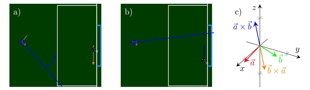
Our next example aims to help in solving a fundamental problem which presents itself to the goalkeeper, namely which part of the goal it should be defending. Our AI tries to predict from where and in which direction the next shot is going to be. In many simple situations it defaults to the assumption that the robot, which is currently in possession of the ball, will shoot in the direction it is currently looking at. This leads to an obvious attack strategy: rotate with the ball in the direction opposite to where the keeper is moving. Then use the time the keeper needs to break and change directions to shoot into the free corner and hopefully score a goal (see fig. 10).

One way to counteract this strategy would be to restrict the keeper to an area around the center of the goal while the opponent is still rotating with the ball. As an added benefit, this prevents the keeper from building up too much speed from which it would need to break down again to change the direction. The general rationale behind this behavior is that it is fundamentally impossible to know where the opponent will try to shoot while it is still rotating. Therefore, the keeper needs to be able to defend both sides of the goal in this situation.

At this point, one encounters a similar problem to that explained in section 4.4. How does one properly detect rotations? Naively calculating the angular velocity by finite differences yields the same problems as before. Luckily, a similar trick can be found to circumvent this. One can make use of the fact that the cross product of consecutive vectors will point in opposing directions depending on whether the second vector is rotated from the first clockwise or counter-clockwise (see fig. 10). Due to the small angle approximation $\sin(x) \approx x$ for small x, the length of the cross product will be approximately linear in the angle with which the vector has rotated. By averaging the previous n cross products between consecutive shot predictions $\boldsymbol{w}$

$$\frac{1}{n} \left| \sum_{j=0}^{n-1} \boldsymbol{w}j \times \boldsymbol{w}{j+1} \right|,$$

large results are obtained when the prediction is continuously rotating in one direction while fluctuations caused by noise will be uncorrelated and therefore cancel each other.

For the use case in our AI the shot predictions are given by vectors of unit length. With a threshold of 0.01 and a buffer size of n=8 we are able to reliably detect the rotation and block the shots that are described above as long as they are not happening too close to our defense area.

4.6 Example 3: Detecting accelerations or decelerations

For our last example let us consider this situation. We are in possession of the ball and want to take a shot at the goal. Let's further assume that we have more than enough time to confuse the opponent keeper before actually shooting. We could for example try to lure the keeper into a specific corner of the goal and then shoot into the other one. One could now ask what the best time would be to start aiming for the other corner.

We argue now that the best time is the moment at which the opponent keeper starts to decelerate on its way to the position we want to lure it to. The reasoning behind this is that you don't gain any more time for the shot by further luring the keeper into the corner, since it will be decelerating either way.

This argument necessitates a tool to reliably predict whether a robot is decelerating or not. The naive approach of using finite differences to estimate the acceleration is even more problematic here, as taking the numerical derivative twice exacerbates the noise problem. The approach we present here is based on trend analysis. Since we only want to know whether the keeper is decelerating or not and don't care by how much, we can use the Kendall tau [17] to decide whether the trend in velocities is rising or falling.

Trend analysis by the Kendall tau is based on counting so-called concordant and discordant pairs of data. A pair of data points ($x^i$ , $y^i$) and ($x^j$ , $y^j$ ) is said to be concordant if the sorting order of both the x and y components agree, i.e. if both $x^i < x^j$ and $y^i < y^j$ or both $x^i > x^j$ and $y^i > y^j$ . Otherwise, the pair is said to be discordant. Ties are ignored for now, as they are practically irrelevant for floating point data. The Kendall tau for $n^c$ concordant and $n^d$ discordant pairs out of $n$ data points is now defined as

$$\tau = \frac{n_c - n_d}{\binom{n}{2}} \in [-1, 1].$$

It quantifies the certainty with which a rising trend (for positive values) or a falling trend (for negative values) can be attributed to the data. For example, strictly monotonically increasing data will have $\tau$ = 1 and strictly monotonically decreasing data will have $\tau$ = −1. Data where the y values fluctuate randomly around some constant will have $\tau$ ≈ 0.

In our experience a buffer size of $n$ = 10 and a threshold of −0.7 with a hysteresis region of half-width 0.2 works reasonably well for detecting when the keeper starts to decelerate.

5 Conclusion

This paper describes the design of our robot covers, as well as simple and costeffective manufacturing process. It compares our design to several other cover designs and lists advantages and disadvantages of it.

Furthermore, it presents a simple electrical simulation of the kicker and compares it to measurements of the kicker we use in our robots. However, there is still some future work needed to create a more detailed simulation that can be used to optimize the electrical and mechanical parameters of the kicker.

In addition, the strategy section contains statistical methods for dealing with noisy data from the vision system and motivates them with multiple examples.

References

1. Abiyev, R.H., Akkaya, N., Arici, M., Cagman, A., Huseyin, S., Musaogullari, C., Turk, A., Say, G., Yirtici, T., Yilmaz, B., Aytac, E.: NEUIslanders Team Description Paper RoboCup 2018. (2018)
2. Silva, C., Alves, C., Martins, F., Machado, J.G., Damurie, J., Cavalcanti, L., Vinicius, M., Sousa, R., Rodrigues, R., Fernandes, R., Morais, R., Araujo, V., Silva, W., Barros, E., Bassani, H.F., de Mattos Neto, P.S.G., Ren, T.I.: RoboCIn 2020 Team Description Paper. (2020)
3. Cosenza, C.S., Couto, G.C.K., Germano, L., Correa, L.G., de S. Barreira, L., de Farias, L.D.P., Rodrigues, L.R.L., de Melo, J.G.O.C., Bozza, M., de Souza, M.P., de Oliveira, N.S.M.M., Silveira, O.C.B., dos Reis, R.P., de Souza, R.P., Dias, S.G.S., Nihari, Y., Rosa, P.F.F.: RoboIME: From the top of Latin America to RoboCup 2018. (2018)
4. Bergmann, P., Engelhardt, T., Gareis, E., Hahn, U., Heineken, T., Hopf, V., Möser, R., Mutter, F., Schmid, M., Schmidt, M., Stadler, M., Wendler, A., Wiedmann, M.: ER-Force 2023 Extended Team Description Paper. (2023)
5. Nikolaus Mitchell, Hunter Scott, Stoian Borissov, Eric Huang, Ryo Osawa, and Matt Barulic: Robojackets 2013 team description paper. (2013)
6. Omid Najafi Koopai, Mohammad Ali Ghasemieh, Mehran Khanloghi: Immortals 2018 team description paper. (2018)
7. Zickler, S., Laue, T., Birbach, O., Wongphati, M., Veloso, M.: SSL-vision: The shared vision system for the RoboCup Small Size League. In: Robot Soccer World Cup, Springer (2010) 425–436
8. Huang, Z., Chen, L., Li, J., Wang, Y., Chen, Z., Wen, L., Gu, J., Hu, P., Xiong, R.: ZJUNlict Extended Team Description Paper for RoboCup 2019. (2019)
9. Browning, B., Bruce, J., Bowling, M., Veloso, M.: STP: Skills tactics and plays for multi-robot control in adversarial environments. Proceedings of the Institution of Mechanical Engineers, Part I: Journal of Systems and Control Engineering 219 (2005) 33–52
10. Rodríguez, S., Rojas, E., Pérez, K., López, J., Quintero, C., Calderón, J.M., Peña, O.: STOx's 2015 Extended Team Description Paper. (2015)
11. Bai, C.Y., Gong, W., Hers, B., Hsieh, B., Iaco, R.D., Ju, Y.Z., Jury, B., Long, B., Lu, K.L., Petrie, J., Tonks-Turcotte, K., Xie, C., Yang, D., Zaari, R., Zhang, K., Zhang, Z.: 2017 Team Description Paper: UBS Thunderbots. (2017)
12. Cunningham, A., Posey, S., Johnson, B., Borissov, S., Gendreau, A., Mitchell, N.: RoboJackets 2011 Team Description Paper. (2011)
13. Hoffmann, M., Lieret, M., Kerschbaum, S., Eischer, M., Nordhus, P., Hauck, A.: ER-Force Team Description Paper for RoboCup 2013. (2013)
14. Mehrabi, V., Koochakzadeh, A., Poorjandaghi, S.S., Pour, S.M., Sheikhi, E., Saeidi, A., Kaviani, P., Saharkhiz, S., Pahlavani, A.: Parsian Extended Team Description for Robocup 2012. (2012)
15. Poudeh, A.G., Nejad, V.K., Dalvand, A., Doost, A.R., Keivanani, M.A., Shirazi, H., Esmaeelpourfard, S., Rashnozadeh, F., Mosayebi, S., Naeini, M.K., Adhami-Mirhosseini, A.: MRL Extended Team Description 2019. (2019)
16. Bergmann, P., Engelhardt, T., Heineken, T., Hopf, V., Schmid, M., Schmidt, M., Schofer, F., Schuh, K., Stadler, M.: ER-Force 2022 Extended Team Description Paper. (2022)
17. Kendall, M.G.: A new measure of rank correlation. Biometrika 30(1-2) (1938) 81–93