KIKS Extended Team Description for RoboCup 2024
Ryuto Tanaka, Daichi Miyajima, Hayato Mitsuda, Kazuaki Harada, Mizuki Nonoyama, Futa Sato, Haru Niimi, Takahiro Miyauchi, Chihiro Takanashi, Yuzuki Hachisuka, Chiaki Naito, Yota Dori, Hirokazu Komatsu, Toko Sugiura
Nat'l Inst. of Tech., Toyota College, 2-1 Eisei-cho, Toyota, Aichi 471-8525, Japan; Kindai University, 1 Takayaumenobe, Higashihiroshima, Hiroshima 739-2116, Japan
https://www.ee.toyota-ct.ac.jp/staff/sugi/RoboCup.html
Abstract In this paper, we mainly describe the improvements and studies of the software system of SSL Team KIKS, which will participate in RoboCup 2024 Eindhoven. We will introduce the improvements of the educational board for new participants and the control results using IMU and current sensors. In addition, the effectiveness of the robot's self-position estimation was verified using rotary encoders and a Local Vision camera to support the Global Vision method. Furthermore, all matches of the Div-A knock-out stage of RoboCup 2023 were analyzed.
Keywords: RoboCup, small size league, autonomous robot, global vision, engineering education
1 Introduction
Team KIKS has been continuing its efforts to develop higher performance hardware and smarter AI systems. Currently, the team is mainly studying software improvements to enhance the robots' control performance. In another experiment, we used a Local Vision and encoders introduced last year to experiment with motion control based on the robot's own decisions, without using Global Vision. On the other hand, minor changes will be made to the previous robots and the number of robots will be increased for the 2024 competition. In addition, we analyze the RoboCup 2023 games and discuss the introduction of offside rules. The details of the experiments are described in each section.
2 Electrical system
This chapter describes the studies performed after the RoboCup 2023 regarding the introduction of electronic circuits and sensors.
2.1 Development of educational boards for new participants
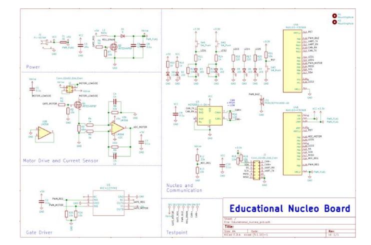
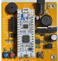
In recent years, the KIKS team has accepted students in the first grade (15-16 years old) who have just graduated from junior high school. They usually do not have sufficient knowledge of robotics and have never taken classes on it. Therefore, after teaching them a series of theories about circuits and the characteristics of their elements, we provided them with educational boards equipped with microcontroller boards and carried out basic education on circuits and embedded program development. The educational board provided was an original developed by our team. Figure 1 and 2 show a photograph and a circuit diagram, respectively. The circuit diagram incorporates a current sensor with a boost chopper circuit and a differential amplifier circuit to help deepen understanding of electronic circuits. In addition, a serial communication environment that can be realized with the F303K8, including UART and CAN, was also implemented. Through this board, students can experience the development of basic embedded systems such as soldering chip components, reading analog sensors, controlling motors, and board-to-board communication. Furthermore, the final goal is to obtain basic and preliminary knowledge of electronic circuits and C programming, as well as debugging skills through these experiences.
2.2 Robot status indicator
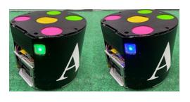
The total elapsed time for HALT associate with Robot Substitution in all SSL matches of RoboCup2023 was 296 minutes [1]. It was equivalent to approximately 12 % of the total match time. KIKS carried out Robot Substitution of 142 times, mainly to remove robots that had lost control due to poor communication or to replace batteries. In order to make the match progression more smoothly, it is necessary to quickly identify the robot with abnormalities and to reduce the time required for substitution. Therefore, we introduced an indicator that displays the robot's status using a full-color LED shown in Fig. 3. Depending on the robot's status, the indicator lights up or blinks in several colors as shown in Table 1.
Color corresponding to the problem
| Problem symptoms | Color of Indicator |
|---|---|
| None | White |
| Low battery | Purple |
| Communication Error (internal) | Green |
| No connection for AI server | Blue |
3 Software system
(blank section header)
3.1 Verification of velocity estimation using encoder, IMU and current sensors
Our robots are controlled by a target velocity sent from a server. By making the robot operate precisely in accordance with the target velocity, we can improve all of its movements, such as catching a ball or defensive performance of a goalie. At present, however, KIKS robots are not able to follow their velocity with sufficient precision. This is due to the fact that the only device used for the velocity estimation is an encoder, which cannot recognize the influence of wheel slip and other factors, and thus cannot obtain the correct velocity. The new circuit board developed two years ago [2] is equipped with an IMU to measure the acceleration of the robot (in three dimensions) and a current sensor to measure the phase current of the motor, but these sensors have not been used in previous games. In this section, we describe an improvement that uses these sensors for more accurate velocity estimation.
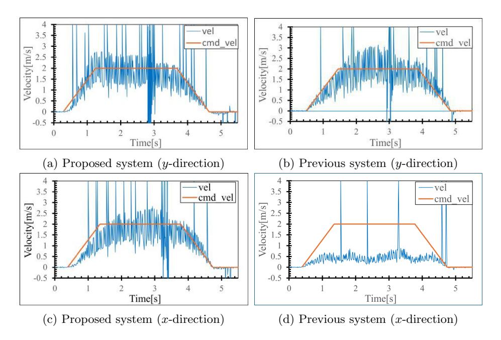
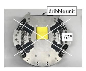
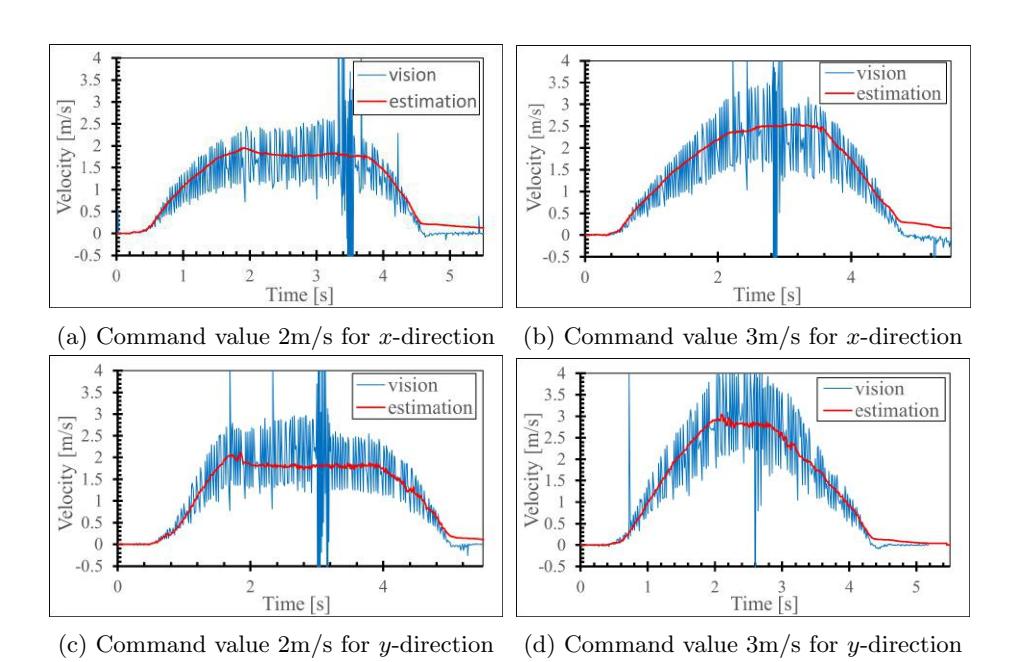
Evaluation of velocity-following performance In order to evaluate the velocity estimation performance of the proposed system, we compared the actual velocity of the robot to a command velocity with that of previous system. The command velocity was a trapezoidal velocity with an acceleration of 2m/s$^2$ and a maximum velocity of 2m/s in the $y$- and $x$-directions, respectively, and the actual velocity of a robot was measured from vision system. These results are shown in Fig. 4(a)~(b). The y-direction speeds shown in Fig.4(a) and (b) indicate that both the previous and proposed systems are able to follow the commanded velocity. For the acceleration situation, however, the proposed system is able to sufficiently follow the given velocity command without delay, whereas the previous system follows the command with a delay. This is a result of the detection and compensation of wheel slip during acceleration by the IMU in the proposed system. On the other hand, for the $x$-direction in Fig.4(c) and (d), the velocity following performance of the previous system using only the encoder was significantly lower. The actual motion of the robot was not straight forward, but went around in a circle. In the proposed system, the acceleration following performance is slightly worse than that in the $y$-direction, but the velocity following performance is almost there. One of the reasons why the characteristics in the $x$-direction are worse than those in the $y$-direction could be the slipping of the wheels. As shown in Fig. 5, the wheel arrangement of our robot is not symmetrical 45° in the front-back and left-right directions. In particular, movement in the $x$-direction is more likely to cause slipping because the angle between the axis of the wheel and the direction of movement is small. In addition, regarding the $x$-direction, in the previous system, slipping occurs not only during acceleration, but also during constant velocity movement. The velocity estimation performance at high velocity movement and in the $x$-direction, however, is not sufficient due to constant slipping of the wheels. In the next section, velocity following performance will be investigated.
3.2 Verification of self-positioning control by robot
Global Vision (GV) system is very advantageous for tactical decision making because it provides fast positional information of the ball and the opponent or allied robots. On the other hand, it has the following problems.
- (1) Robot or ball may not be correctly recognized by GV
- (2) There is a delay until the GV recognizes the robot and the velocity command reaches the robot from the server.
- (3) Since the commands to the robot are transmitted wirelessly, noise superimposition or missing commands may occur.
When above problems occur, the control performance of the robot will be lower. In this section, we describe the control using the robot's odometry function (using an encoder attached on the motor) and a small local vision (LV) camera mounted on the robot. The robot performs its self-position estimation and generates velocity commands, and a high precision motion control method using only LV is investigated.
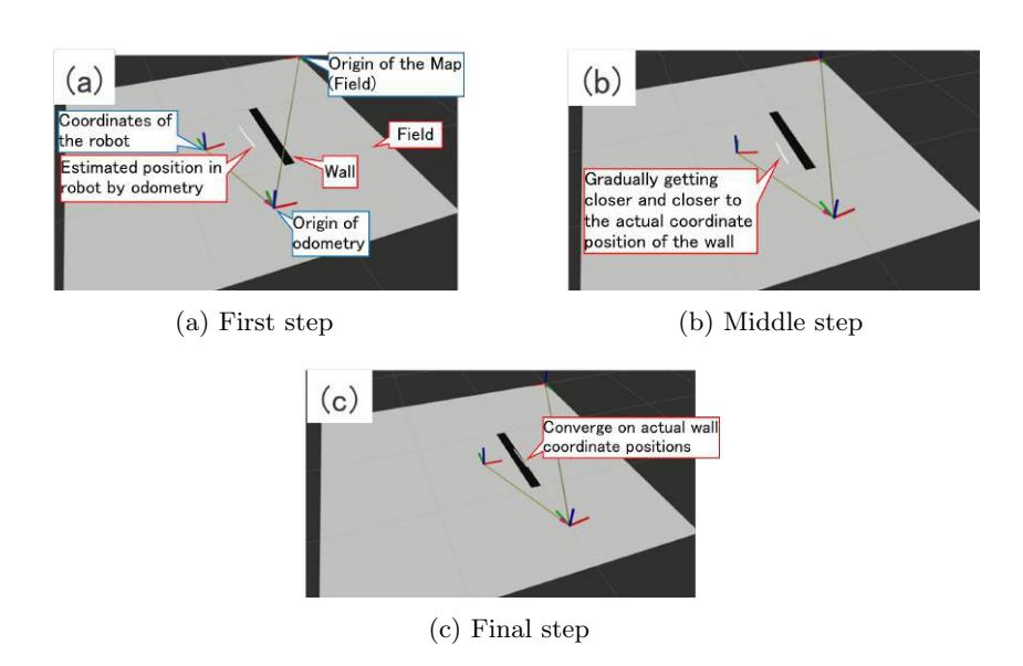
Verification of the introduction of AMCL method AMCL (Adaptive Monte Carlo Localization) is a method that estimates the current position as a probability distribution based on the amount of movement, and derives the most probable position coordinates based on scan data from LiDAR (Light Detection And Ranging) devices (e.g., distance to a wall) and map data. In this study, the ROS2 (Robot Operating System 2) package nav2 amcl was used, and the parameter robot model type was executed as nav2 amcl::OmniMotionModel[5]. When using AMCL, it is necessary to provide information on the surrounding environment (presence of robots and walls) as a point group, and LiDAR (Light Detection And Ranging) is normally used. In this study, however,an LV camera is used, and the camera image must be converted to a point group. Since it is defined that the field surface is green and the outer wall is black for color in SSL [6], the images are filtered and then edge detection is performed. All of the detected edge pixels are converted into a plausible point group and use as pseudo LiDAR scan data. In the experiment, the map data of the wall was given to the robot in advance, and the robot was placed at a location away from the position coordinates recognized inside the robot. Then, we verified whether the robot could converge the position coordinates to the correct coordinates using only the LV camera. No GV was used in this experiment.
Results and discussion Figure 7(a)-(c) show the results of the experiment. The white surface represents the field, the black thick line indicates the actual wall, and the white line indicates the position of the wall as perceived by the LV camera. The red, green, and blue lines in each figure show the x-, y-, and zaxes from the origin, respectively. The gray lines represent vectors from the map origin to the odometry origin and from the odometry origin to the robot position, respectively. Figure 7(a) shows the initial state, i.e., that there is a gap between the coordinate position recognized by LV and the actual (accurate) position of the wall. This corresponds to the fact that the position coordinates including errors due to odometry are recognized inside the robot. (b) shows how the actual wall position and the wall position recognized inside the robot gradually match by the wall recognition by LV and the correction process by AMCL. Finally, as shown in (c), the actual wall position and the position recognized by the robot matched and converged. As described above, it was shown that it is possible to recognize accurate position coordinates inside the robot if corrections are performed by AMCL while the wall is recognized by LV.
3.3 Evaluation of ball-following based on consensus control system
A Multi-Agent System (MAS) is a distributed system in which multiple autonomous robots communicate with each other [7], [8], [9]. MAS can be useful when a centralized control system with a single server cannot support it, as in the case of Vision Blackout in SSL. In this section, we describe a basic study on ball-following control using consensus control, one of the MAS methods.
Mathematical model for ball-following control We consider a mathematical model for the ball-following control. Here, we assume that the positions of a ball and a robot are located on a one-dimensional line. Let the positions of the ball and the robot be $x_1(t) \in \mathbb{R}$ and $x_2(t) \in \mathbb{R}$, respectively. The ball-following model can be described by the following ordinary differential equations (ODEs):
$$\frac{d}{dt}x_1(t) = f(t) \quad a.e. \quad t \ge 0, \frac{d}{dt}x_2(t) = a_{21}(t)(x_1(t) - x_2(t)) + g(t) \quad a.e. \quad t \ge 0,$$
where a function $f \in C([0,T);\mathbb{R})$, T is a time, represents the behavior of the ball and a function $g \in C([0,T);\mathbb{R})$ is the control input that the robot to track the ball. A non-negative continuous function $a_{21}:[0,T)\to\mathbb{R}{\geq 0}$ is a weight coefficient of communication between the robot and the ball. The robot obtains the position of the ball through this communication. Here, we impose the following condition for the coefficient $a{21}(t)$,
$$0 \le m_{21} \le a_{21}(t) \le M_{21}.$$
We consider a condition for the control input g(t) that the robot to reach the ball at a time T > 0. Mathematically speaking, for any time $t \geq 0$ there is a control input g(t) such that the limit holds,
$$\lim_{t \to T} |x_1(t) - x_2(t)| = 0.$$
We obtain the following theorem with respect to the condition for the control input.
Theorem1. For any function $f \in C([0,T);\mathbb{R})$ and $a_{21} \in C([0,T);\mathbb{R})$ satisfying the condition, and for any initial value $x_1(0)$, $x_2(0) \in \mathbb{R}$, the limit holds if and only if the control input $g \in C([0,T);\mathbb{R})$ satisfies the following condition,
$$\lim_{t \to T} \left| x_1(0) - x_2(0) + \int_0^t e^{\int_0^s a_{21}(u)du} (f(s) - g(s)) ds \right| = 0.$$
For example, we can find one of the control inputs
$$g_c(t) = f(t) + \frac{e^{-\int_0^t a_{21}(s)ds}}{T} (x_1(0) - x_2(0)).$$
Optimal control As we saw in the previous subsection, many control inputs satisfy the condition. Hence, we need to find an optimal control input for the robot to track the ball. That is, the control input has to minimize the sum of the distance between the robot and the ball on the interval [0, T].
Here, we consider a control input that minimizes the following cost function J along solutions to Eq.(1):
$$J[x_2, f, g] = \int_0^T \left(\frac{1}{2} \left(\int_0^t f(s)ds + x_1(0) - x_2(t)\right)^2 + \frac{1}{2}g^2(t)\right)dt.$$
Let the optimal control input and the optimal solution be denoted by $g^(t)$ and $x^(t)$, respectively. Then, $g^(t)$ and $x^(t)$ satisfy the following conditions called Pontryagin's Minimum Principle[10]:
$$\frac{d}{dt}x^(t) = \frac{d}{d\lambda^}H(t, x^(t), g^(t), \lambda^*(t)),$$
$$\frac{d}{dt}\lambda^(t) = -\frac{d}{dx^}H(t, x^(t), g^(t), \lambda^*(t)),$$
$$H(t, x^(t), g^(t), \lambda^(t)) = \min_{g \in G} H(t, x^(t), g, \lambda^*(t)),$$
where G is the subset of the control inputs satisfing the condition, and $\lambda^*(t)$ is the optimal Lagrange multiplier. Moreover, a Hamiltonian H is defined as follows:
$$H(t, x_2(t), g(t), \lambda(t)) = \frac{1}{2} \left( \int_0^t f(s)ds + x_1(0) - x_2(t) \right)^2 + \frac{1}{2}g^2(t) + \lambda(t) \left( a_{21}(t) \left( \int_0^t f(s)ds + x_1(0) - x_2(t) \right) + g(t) \right),$$
where $\lambda(t)$ is the Lagrange multiplier.
Applying Eq. (7) to the above H, we obtain the following equations:
$$\frac{d}{dt}x_2(t) = a_{21}(t)\left(\int_0^t f(s)ds + x_1(0) - x_2(t)\right) + g(t),$$
$$\frac{d}{dt}\lambda(t) = \int_0^t f(s)ds + x_1(0) - x_2(t) + a_{21}(t)\lambda(t),$$
$$g(t) + \lambda(t) = 0.$$
Therefore by solving Eqs.(9a)-(9c), it is possible to construct the optimal control input based on the cost function Eq.(6). We put the optimal control input g(t) as $g_o(t)$ satisfying Eqs.(9a)-(9c).
Numerical simulation We will numerically evaluate a ball-following performance of the robot by applying the result above. In order to consider a real situation in soccer games, we extend the result on the 2D plane. We define the positions of a ball and the robot by the vectors $\mathbf{x}_1(t) = [x_1(t), y_1(t)]^T$ and $\mathbf{x}2(t) = [x_2(t), y_2(t)]^T$, respectively. The ball-following model can be also presented as the ODEs (Eq.(1)) on 2D plane, where the behavior of a ball is $f(t) = [f_x(t), f_y(t)]^T$, and the control input is $g(t) = [g_x(t), g_y(t)]^T$. Moreover, we assume that $a{21}(t) \equiv 1$.
In case of 2D plane, we obtain the following control input in the same way as Eq.(5):
$$g_c(t) := \begin{bmatrix} g_{c_x}(t) \ g_{c_y}(t) \end{bmatrix} = \begin{bmatrix} f_x(t) + \frac{e^{-t}}{T} (x_1(0) - x_2(0)) \ f_y(t) + \frac{e^{-t}}{T} (y_1(0) - y_2(0)) \end{bmatrix}.$$
Moreover, we define the optimal control input $g_o(t) = [g_{o_x}(t), g_{o_y}(t)]^T$, which $g_{o_x}(t)$ (resp. $g_{o_y}(t)$) minimizes the cost function $J[x_2, f_x, g_{o_x}]$ (resp. $J[y_2, f_y, g_{o_y}]$) along the solutions to Eqs.(9a)-(9c) with regarding to $x_2(t)$ (resp. $y_2(t)$). We can obtain the optimal control $g_{o_x}(t)$ as follows,
$$g_{o_x}(t) = (\sqrt{2} + 1)(e^{\sqrt{2}t}(F_{1_x}(t) + C_{1_x}) - e^{-\sqrt{2}t}(F_{2_x}(t) - C_{2_x})) + e^{\sqrt{2}t}\frac{d}{dt}F_{1_x}(t) + e^{-\sqrt{2}t}\frac{d}{dt}F_{2_x}(t) - \left(\int_0^t f(s)ds + x_1(0)\right),$$
where,
$$\begin{split} F_{1_x}(t) &= \int_0^t \frac{e^{-\sqrt{2}s}(f_x(s) - 2x_1(s))}{2\sqrt{2}} ds, \quad F_{2_x}(t) = \int_0^t \frac{e^{\sqrt{2}s}(f_x(s) - 2x_1(s))}{2\sqrt{2}} ds, \ C_{1_x} &= \frac{e^{-\sqrt{2}T}(x_2(0) - F_1(0) + F_2(0)) + x_2(T) - e^{\sqrt{2}T}F_1(T) + e^{-\sqrt{2}T}F_2(T)}{e^{\sqrt{2}T} - e^{-\sqrt{2}T}}, \ C_{2_x} &= \frac{e^{\sqrt{2}T}(x_2(0) - F_1(0) + F_2(0)) + x_2(T) - e^{\sqrt{2}T}F_1(T) + e^{-\sqrt{2}T}F_2(T)}{e^{\sqrt{2}T} - e^{-\sqrt{2}T}}. \end{split}$$
By replacing x with y, the optimal control input $g_{o_y}(t)$ is expressed in the same formulation as $g_{o_x}(t)$.
We numerically compare the trajectory of the robot following control input $g_c(t)$ given as Eq.(10) with one following the optimal control input $g_o(t)$ given by solving Eq.(11). In addition, we evaluate the behavior of a ball-following robot in three cases of $T = 500 ,(\text{ms}), 1000 ,(\text{ms}), 3000 ,(\text{ms})$.
Furthermore, we calculate the cost functions $J_c := [J[x_2, f_x, g_{c_x}], J[y_2, f_y, g_{c_y}]]^T$ and $J_o := [J[x_2, f_x, g_{o_x}], J[y_2, f_y, g_{o_y}]]^T$ corresponding to the robot following the $g_c(t)$ and $g_o(t)$, respectively. Here, we put the initial values as $\mathbf{x_1}(0) = [x_1(0), y_1(0)]^T = [0, 0]^T$ and $\mathbf{x_2}(0) = [x_2(0), y_2(0)]^T = [0, 1]^T$. We estimate the trajectory of $\mathbf{x_2}(t)$ in two cases of the behavior of a ball; Case1, $[f_x(t), f_y(t)]^T = [1, 0]^T$; Case2, $[f_x(t), f_y(t)]^T = [\cos t, \sin t]^T$.
![The trajectory of a ball and a robot in case of $[f_x(t), f_y(t)]^T = [1, 0]^T$ on 2D plane (Red, blue, and green lines indicate the trajectories of a ball, a robot following $g_c(t)$, and a robot following $g_o(t)$, respectively).](/tdps/soccer_smallsize__2024__KIKS/_page_10_Figure_2.jpeg)
![The trajectory of a ball and a robot in case of $[f_x(t), f_y(t)]^T = [\cos t, \sin t]^T$ on 2D plane (Red, blue, and green lines indicate the trajectories of a ball, a robot following $g_c(t)$, and a robot following $g_o(t)$, respectively).](/tdps/soccer_smallsize__2024__KIKS/_page_10_Figure_4.jpeg)
4 Game analysis using log data
In recent years, statistical data has been increasingly utilized in real soccer. Objective rather than subjective analysis of the game is becoming more popular, for example, as information is shared with viewers during TV broadcasts. On the other hand, there are some rules in SSL that differ from those in real soccer. Among them, the offside is an important factor that determines the score in real soccer, but it does not take into account in SSL. Therefore, in this section, we will try to discuss them based on objective data of goal-scoring scenes in the knock-out stage of SSL in RoboCup 2023.
4.1 Analyzing method
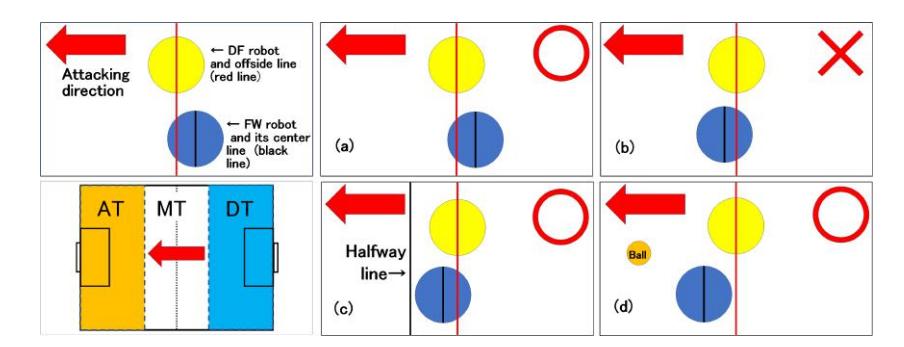
We implemented a measurement function in the team's original GUI and analyzed the log-data from the official logs of SSL. For the shooting scene, we evaluated the shooting position, the position where the attack started (FreeKick position or the starting point of the flow of shooting as a result of stealing a ball from the opponent in the game), and also the offsides. For offsides, assuming that the robot's coordinate point was the center of the circle, we evaluated using the following criteria as shown in Fig.10.
- (1) When a ball is kicked, an attacking robot is offside if it is in front of the second robot from behind of the defending robot and receives the kicked ball directly. (Fig.10 a, b)
- (2) Same as in real soccer, offsides are not taken when the robot is not in an opponent's territory or when the robot is behind the ball. (Fig.10 c, d)
- (3) For the sake of simplicity, offside is only considered when the ball is passed directly.
The data used in the analysis were focused only on Div-A knock-out stage.
4.2 Verification items
(a) Shooting position In Fig 11, we plot all the shooting positions for the 10 games in which a goal was scored. The dotted lines indicate the boundaries of the AT in the field. The legend corresponds to the game numbers in Table 2. Figure12 shows the percentage of goals scored in each of the eight areas. The results in Fig.12 show that the total percentage of shootings in the AT was 82%. Of these shots, 29% were scored from the both sides of the defensive area (Near). Shooting from MT (outside the AT) was classified as Far in Fig. 12. As for the direction along the goal line, it was found that shoots from the area in front of the goal (Center) had the highest success rate (46%) as shown in Fig.12. Figure 11 shows that shoots from the center of the defensive area and from the corners on both sides of the same area are more often resulted in a goal. This may be due to the fact that the defending robots move slowly (carefully) around the corners of the area to avoid entering the allied defensive area.
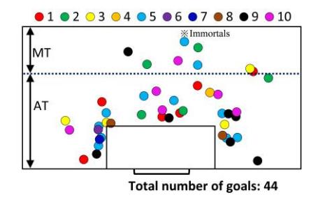
Game score of the Div-A Knock-out stage in RoboCup2023
| Game No. | Winner team | Score | Looser team |
|---|---|---|---|
| 1 | RoboDragons | 6 | 0 ER-Force |
| 2 | Immortals | 5 | 0 RoboTeamTwente |
| 3 | KIKS | 4 | 0 RoboTeamTwente |
| 4 | ZJUNlict | 1 | 0 RoboDragons |
| 5 | TIGERs Mannheim | 10 | 1 Immortals |
| 6 | KIKS | 1 | 0 RoboDragons |
| 7 | Immortals | 1 | 0 ER-Force |
| 8 | TIGERs Mannheim | 2 | 0 ZJUNlict |
| 9 | Immortals | 7 | 0 KIKS |
| 10 | ZJUNlict | 6 | 0 Immortals |
| 11 | TIGERs Mannheim | 0 | 0 ZJUNlict |
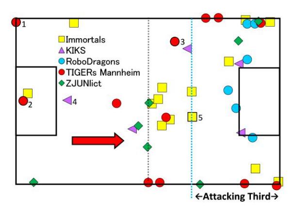
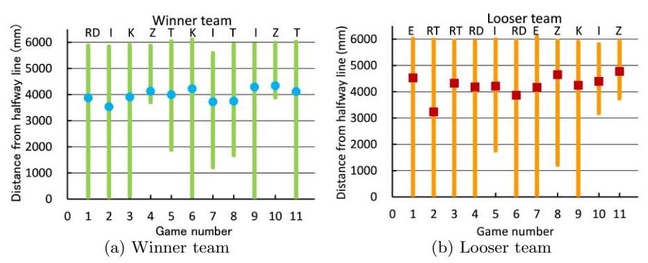
(b) Attacking possession phase (APP) Table 3 summarizes the scores of all Div-A teams in RoboCup 2023. Figure 13 shows the plots of starting points for attack. It can be confirmed that the starting points for attack of the higher-ranked teams cover the entire field area. This suggests that the higher-ranked team made effective use of a large area by moving fast and precisely through the field with a lot of passing. On the other hand, the lower-ranked teams often lose a ball to the higher-ranked teams, and as a result, they may make their starting points for attack only in a limited area of the field.
Total goals for the Div-A teams in RoboCup2023
| Rank | Team | Goals |
|---|---|---|
| 1 | TIGERs Mannheim | 12 |
| 2 | ZJUNlict | 7 |
| 3 | Immortals | 14 |
| 4 | KIKS | 5 |
| 5 | RoboDragons | 6 |
| 5 | ER-Force | 0 |
| 7 | RoboTeamTwente | 0 |
| Total Goals | 44 |
Acknowledgments
The authors wish to express their deep appreciation to N. Fujii, KIKS alumnus for development of main circuit board and firmware. This work was supported in part by Grant-in-Aid from The Nitto Foundation and The Sango Foundation for Education in Japan, respectively.
References
- TIGERs Mannheim, Game Events, https://metabase.tigers-mannheim.de/public/dashboard/2a77fd2f-b8f9-4b34-8b6c-67bdf084b2a8
- Ryoma Mitsuoka, et al., KIKS Extended Team Description for RoboCup 2022; https://ssl.robocup.org/wp-content/uploads/2022/04/2022_ETDP_KIKS.pdf
- Board and firmware of KIKS robots, https://github.com/Nkyoku/phoenix-firmware
- Board and firmware of KIKS robots[In Japanese], https://github.com/Nkyoku/phoenix-firmware/wiki/Control
- ROS navigation: Configuration Guide AMCL, https://navigation.ros.org/configuration/packages/configuring-amcl.html
- Rules of the RoboCup Small Size League, https://robocup-ssl.github.io/ssl-rules/sslrules.html
- M. Mesbahi and M. Egerstedt, Graph Theoretic Methods in Multiagent Networks, Princeton, 2010.
- R. Olfati-Saber, J. A. Fax, and R. M. Murray, Consensus and cooperation in networked multi-agent systems, Proceedings of IEEE, Vol. 95, No. 1, pp. 215-233, 2007.
- R. Olfati-Saber and R. M. Murray, Consensus problems in networks of agents with switching topology and time-delays, IEEE Transactions on Automatic Control, Vol. 49, No. 9, pp. 988-1001, 2004.
- E. D. Sontag, Mathematical Control Theory, Springer, 1990.