TIGERs Mannheim
Nicolai Ommer, André Ryll, Michael Ratzel, Mark Geiger
Department of Information Technology Baden-Württemberg Cooperative State University, Coblitzallee 1-9, 68163 Mannheim, Germany
Abstract This paper presents latest improvements of ball control and path planning algorithms of TIGERs Mannheim, a Small Size League (SSL) team intending to participate in RoboCup 2024 in Eindhoven, Netherlands. This year, the ETDP will focus on state-of-the-art methods for dribbling a ball and the employed control architecture. Furthermore, many implementation details and improvements to our trajectory-sampling-based path planning are depicted. This includes generating and executing trajectories, handling dynamic obstacles, and dealing with corner cases.
1 Robot Hardware Updates
Over the last two years, we only made minor improvements to our existing v2020 robots. The dribbler material and shape has been changed. Our v2020 generation is still performing very well and currently does not require any major updates. All electronics have remained unchanged. The full mechanical and electrical specifications can be found at the end of this section in table 1. A detailed description of our v2020 hardware can be found in [1,2]. The last update of the dribbler design introduced a 2-DoF damping as shown in [3].
Independent of the damping, the design had two issues with the dribbling bar. Firstly, the molded polyurethane was susceptible to abrasion from the ball. Secondly, the spiral shape was a weak point and the spiral quickly gone due to abrasion. To improve the dribbling bar we moved to a flat one without a spiral on it. Furthermore, we switched to a 3D-printed TPU material with a shore hardness of 60A. This is a soft material which is difficult to print but offers great traction on the ball. The 3D-printing process also offers much faster tests with other shapes because we do not need to make new molds every time. The diameter of the new dribbling bar is 14 mm. Although we lose the ability to center the ball without the spiral shape we accepted this drawback in favour of a more robust dribbling bar.
Table 1: Robot Specifications
| Robot version | v2020 |
|---|---|
| Dimension | Ø178 x 148 mm |
| Total weight | 2.62 kg |
| Max. ball coverage | 19.8 % |
| Locomotion | Nanotec DF45L024048-A2, 65W, Direct Drive |
| Wheel diameter | 62 mm |
| Encoder | iC-Haus iC-PX2604 + PX01S, 23040 ppr [4] |
| Dribbling motor | Moons' Industries ECU22048H18-S101, 55W |
| Dribbling gear | 1 : 1 : 1 |
| Dribbling bar diameter | 14 mm |
| Kicker charge | 3600 µF @ 240 V (103.68 J) |
| Chip kick distance | approx. 3.6 m |
| Straight kick speed | max. 8.5 m/s |
| Microcontroller | STM32H743 @400 MHz [5] |
| Sensors | Encoders, Gyroscope, Accelerometer, Compass, Camera |
| Communication link | Semtech SX1280 @1.3 MBit/s, 2.300 - 2.555 GHz [6] |
| Compute module | Raspberry Pi 3A+ with one forward oriented camera |
| Power Supply | Li-Po battery, 22.2 V nominal (6S1P), 1550 mAh |
2 Dribbling Methods and Control
SSL robots are allowed to control the ball by actively exerting a backspin on it. They must not remove all degrees of freedom of the ball and an area of at least 80% when viewed from above needs to be outside the robot's convex hull. The part of the robot which is exerting backspin is commonly referred to as a dribbling device. These devices appeared first around 2002, which is only 5 years after the league was founded in 1997. Dribbling devices were mainly used with straight forward or backward movement only, as they had little lateral control of the ball. Nevertheless, this allows to pull back the ball from opponents and it is essential during ball placement procedures (introduced 2017 and mandatory in division A since 2018).
Dribbling got more advanced in 2015 when team CMDragons introduced dribbling while turning [7]. A circular path is followed to pass around a single opponent. Because of this skill, among other things, CMDragons won the world championship in 2015. The next step of dribbling device and ball control evolution happened in 2018 when team ZJUNlict demonstrated outstanding movement abilities with the ball. Their so called break skill was able to move with the ball on arbitrary paths, not limited to circular movement [8]. This led to two consecutive world champion titles in 2018 and 2019 for them.
Especially the achievements in recent history show the importance of a good dribbling devices and ball control to become a top team of the SSL. Section 2.1 describes our current dribbler design and two common methods to control the ball. Section 2.2 gives a detailed description of the motor controller used for successful ball handling.
2.1 Dribbler Design
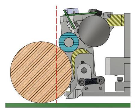
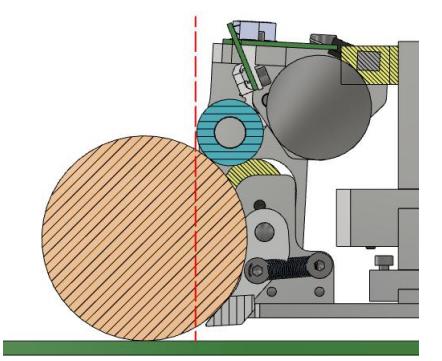
Figure 1 shows the dribbler design of our current v2020 robot generation at two different states. The forward dribbler position is the default position when the robot is not in contact with the ball or when it just made contact. In this state, the ball only has two contact points: with the dribbling bar and with ground. The rearward dribbler position is limited by the chip shovel position. In this state there is an additional contact point between ball and chip shovel. Over the full range of movement the robot does not violate the coverage rule as indicated by the dashed vertical line.
2.2 Dribbler Motor Control
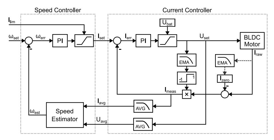
Figure 2 details the control architecture of our dribbler motor. The motor itself is a brushless DC (BLDC) motor with three hall sensors. The three motor windings are energized according to the common 6-step commutation scheme. This is the simplest mode of control for a BLDC motor and results in characteristics and mathematical model equivalent to that of a brushed DC motor. Its main drawback is a small torque ripple as the rotating magnetic field is only adjusted six time per electrical revolution.
In addition to the hall sensors there is one low-side shunt sensor for current measurements. The shunt circuit has a voltage offset to allow bidirectional measurements (accelerating and braking motor). Our dribbling motor is not equipped with an encoder.
3 Path Planning
Path planning is a common problem in the SSL and in robotics in general. A lot of work has been published about this already. In 2019, we described our novel trajectory-sampling-based path planning approach in detail [10], which we started to develop and use in 2015 already. Many teams were using an RRT-based approach back then. In 2020, team ER-Force changed their path planning from an RRT to a similar trajectory-sampling-based approach [11]. In 2023, team RobôCIn compared our solution and that of ER-Force and based their own implementation on that work [12].
Since the last publication in 2019, we have tuned the path planning implementation further. While the basic idea is still the same, much of the original implementation has changed. This chapter describes our current implementation and points out some differences that we applied since our last publication.
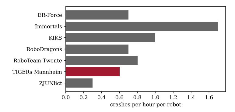
With our approach, we committed about 3 fouls due to collisions where our robot was significantly faster than the opponent (henceforth called crash) on average per match during RoboCup 2023. Figure 3 shows the number of crashes, normalized to the game time and the total number of robots on the field. We achieved the second lowest number of crashes following behind ZJUNlict.
3.1 Overview
The following sections describe our current implementation in detail. The code can be found in our open-source release, see section 4.
Path planning is initiated by a specific skill, the MoveToSkill. It is performed individually and independently for each robot with the following steps:
- Generate a list of obstacles for this bot: Each robot may have individual requirements for path planning. A supporter wants to keep a larger distance to the ball, while an attacker needs to touch it. A defender wants to respect opponents in a more defensive / aggressive way than other robots. Details on how obstacles are modeled can be found in section 3.5.
- Create and adapt the path finder input: The input to the path finder consists of the robot's current 2D position and velocity, the robot's movement constraints, like maximum velocity and acceleration, the list of obstacles from the previous step and the target position. Both, the target position and the list of obstacles are adapted in this step to handle some special cases, as outlined in section 3.7.
- Find a path: The path finder will return a path finder result, consisting of the trajectory to be executed and a list of collisions along its path. Collisions consist of the obstacle and the first collision time. Sections 3.2 and 3.3 describe the process of generating trajectories and finding collisions along the path and section 3.4 describes how resulting path finder results are accepted or rejected.
- Execute the trajectory: Based on the returned path finder result, the Move-ToSkill will either execute the trajectory, or perform a fast brake, if a collision is imminent. This is outlined in section 3.6.
3.2 Generate Trajectories
The basic approach is straight forward: First, create a trajectory from the current state to the target position. If its path is acceptable, return it. Else, iterate through a finite list of intermediate targets. For each intermediate target, create a trajectory from the current state to the intermediate target. Next, step over the resulting trajectory in discrete time steps tintermediate = 200 ms and create a new trajectory consisting of two parts. The first part is the intermediate trajectory with an upper time limit of tintermediate, the second part is a new trajectory with the initial state of the intermediate trajectory at tintermediate and the final target position. So far, we never created more than one intermediate target for our trajectories. This was sufficient for our use cases. However, it would be an option if more fine-grained paths are needed.
The way of generating the intermediate targets has not changed much in recent years. We still have two different implementations. One that generates a finite list of random targets and one that generates a systematic list. Currently, we use the random-based implementation with five targets. Having such a small number of intermediate targets is acceptable, because we run path planning continuously every frame (about every 10 ms) and can thus eventually find a good path. Additionally, the target from the previous iteration is also added to the intermediate targets. This caches good results and stabilizes the resulting path over time.
Initially, we always calculated paths for all intermediate targets and selected the best one. Now, we choose the first acceptable path and stop. This reduces the overall runtime at the cost of not finding a potentially faster path. With this lazy approach, the order of the intermediate targets has become relevant, so for the random-based implementation, we sort the targets by the angle between current position to target and current position to intermediate target, smallest first. This favors paths pointing towards the target.
3.3 Finding Collisions Along a Trajectory
We apply a simple iterative approach, but also added several optimizations. Basically, we step over a given trajectory and for each time step t, we iterate over all obstacles to check if there is a collision.
In the initial implementation, we used fixed time steps and a binary collision result (colliding or not colliding). In the current implementation, the time steps are dynamic and the obstacles return the distance to the currently checked point. This enabled two improvements. First, the next time step can now be calculated based on how close the closest obstacle is. This can reduce the total number of collision checks significantly. Second, we can apply an extra margin between obstacle and robot. We chose a dynamic margin depending on the robot velocity $v^t$ at the given time step, defined by
$$m = \left(\frac{\min\left(v_{max}, v_t\right)}{v_{max}}\right)^2 * m_{base} \tag{4}$$
with vmax = 3 m/s and margin mbase = 0.2 m. This way, a robot can drive very close to an opponent robot, when slow, but considers an appropriate safety distance when driving fast.
3.4 Accepting or Rejecting Path Finder Results
The Small Size League is very fast and competitive. The best path is not necessarily the fastest one without a collision. We cannot be too careful, because then the opponent may catch the ball before us. Most obstacles are moving robots that can change their direction any time, so the situation has to be reevaluated every frame. Caring about collisions which happen one second in the future are just not worth to consider. However, this is not true in general. There are some static, motionless obstacles like the field boundary and the penalty area. On the other hand, moving obstacles can also be categorized into different behaviors. For our own robots, we know very well, where they will move along. Movement of opponent robots has to be estimated, while avoiding to be pushed or otherwise influenced by the opponents.
Our solution to those specifics are two acceptors, one for moving obstacles and one for motionless obstacles. They are applied to a path finder result and their output is binary: accepted or rejected.
Since last RoboCup (2023), we tuned the moving obstacle acceptor to more reliably intercept a ball before the opponent. Previously, our own robots got too nervous about a crash with the opponent ball interceptor and thus lost the ball against it. The optimization has been successfully evaluated in our simulation.
3.5 Modeling Obstacles
In practice, an obstacle is not just a simple geometric shape. That's why we have several different implementations for different kinds of obstacles. Some consider the current time on the trajectory to account for moving objects. For the field border and penalty area, we have specific obstacles for their geometric shape. Our own robots are modeled by their current trajectory. If they have no trajectory (because they perform some special skill, or because they are broken/off), they are instead modeled by a simple tube shape, which is constructed by position and velocity of the robot. Opponent robots have two different obstacle types that depends on the desired aggressiveness. If we want to be more aggressive, we only assume constant velocity over a short time window, otherwise we expect that robots will accelerate up to a certain maximum velocity.
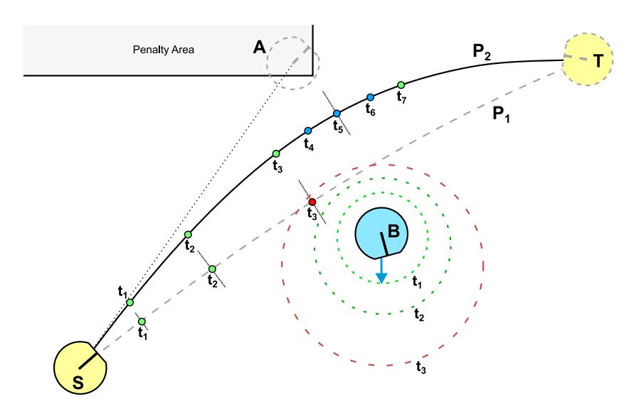
For that, we calculate a circle $r_{dyn}$ depending on time t that defines the area in which the robot could potentially move within this time based on its movement limits. Figure 4 visualizes such an opponent obstacle for multiple time steps. The radius $r_{obstacle}$ and circle center $\vec{p}_{obstacle}$ is calculated with equations (5)-(8).
$$t_{c} = \begin{cases} 0 & \text{for } t < 0 \ t_{max} & \text{for } t > t_{max} \ t & \text{otherwise} \end{cases}$$
$$r_{dyn} = \frac{|f_{+}(t_{c}) - f_{-}(t_{c})|}{2}$$
$$\vec{p}{obstacle} = \vec{p}{op} + [\vec{n}{op} \cdot (f{-}(t_c) + r_{dyn})] \tag{7}$$
$$r_{obstacle} = r_{op} + r_{dyn} \tag{8}$$
$f_{+}$ and $f_{-}$ are the 1D bang-bang trajectories from position zero to positive and negative infinity with the current opponent speed and its velocity and acceleration limits, $\vec{p}{op}$ is the current opponent position, $\vec{n}{op}$ is the current opponent normalized move direction and $r_{op} = 0.09 , m$ is the robot radius. The limits can be adapted to individual opponents, but are usually around $3 \frac{m}{s}$ and $3 \frac{m}{s^2}$. The maximum time $t_{max}$ is set to about 0.5 s, which allows for enough lookahead to react to direction changes of opponents. A higher maximum time results in larger obstacles and thus longer paths. A small tweak is applied to this obstacle to make it less pessimistic. Instead of a circle, only a tube is created. The width of the tube is the robot width and the length is the circle radius. Additionally, for non-moving robots, the dynamic radius is set to zero, effectively reducing the obstacle to a small circle. Without this tweak, our robots would circumvent opponents widely, as they expect them to accelerate in any direction soon.
The ball is modeled by its ball trajectory. If it would simply be modeled with a tube from start to the point where it will stop, this would create a wall across the field that robots could not cross easily, so modeling the ball by time is quite important.
For ball placement, a virtual ball is modeled, as if it would be kicked to the placement position now. This also avoids the wall issue.
3.6 Executing a Trajectory
Executing the trajectory is generally straightforward. Our robots require a target position as input. We take the next (intermediate or final) target position from the trajectory and send it to the robot every frame.
However, before the trajectory is applied, the MoveToSkill will check if it is safe to do so. The trajectory may have a collision and reports the time until the first collision will happen. The skill will calculate if it can reduce the robot velocity to a safe amount before hitting the obstacle. If it is still safe, the path is applied. Otherwise, the skill brakes until it is safe again. The skill will use a larger acceleration for braking, than the path planning considers. This makes it more likely to actually brake in time.
Incorporating the emergency brake feature into the skill offers several advantages. Our current bang-bang trajectories lack the ability to differentiate between acceleration and braking, yet the robots demonstrate a significantly faster braking capability compared to acceleration. Consequently, addressing this within path planning proves challenging. Additionally, planning a path with a reduced brake acceleration enables us to account for inaccuracies and devise a more risky trajectory.
3.7 Handling Special Cases
There are some special cases that have to be dealt with in practice.
Target is inside an obstacle If the target is located inside an obstacle, no collision free path could ever be found and the robot could never reach the target. We apply a simple trick: We adapt the target such that it is as close as possible to the original target, but not inside the obstacle. Each obstacle has its own implementation for this adaptation, but it is usually just the closest point outside.
Robot is inside an obstacle Similar to the previous scenario, if the robot is already within an obstacle, all paths would inevitably result in a collision. To accommodate this issue, we do two things. First, we remove all obstacles that the robot is in. Additionally, for some obstacles it is not sufficient to just ignore them. For example, we do not want a robot to drive through the full penalty area, just because it accidentally slightly got into it. Another situation is, when two robots are close to each other. Removing the obstacle may result in pushing, if the robot wants to move through the other robot. For those reasons, the target position is adapted just like for the previous case, but this time, a target is chosen that moves the robot out of the obstacle first. This is usually a point towards the closest point outside, but further outside, so that the robot is moving out fast.
A challenge with this approach is to handle multiple overlapping obstacles. Currently, we adapt the destinations sequentially in one run through the list of obstacles. We are working on a more robust solution that finds an adapted destination that satisfies all obstacles.
No path was found There is the rare case where all intermediate targets were tried and there is still no acceptable path. Our current approach is to return a trajectory to the current robot position. If the robot is moving, this is a good way to reduce its speed so that eventually, it will find a path again. Also, due to the random sampling of intermediate targets, there is a chance to find an acceptable path over time. The downside of this approach is, that the robot may stop moving completely.
For the future, we have some ideas to improve on this. Instead of using a path to the current position, we could select one of the rejected paths, like the one that brings us the closest to the destination. Also, it might be beneficial to simply brake, when no path was found. This brings the robot to a stop more cleanly and faster (due to higher acceleration, see section 3.6). It is also beneficial for robot control, as the robot position as destination results in an undesirable feedback loop.
3.8 Summary
Since we switched from an RRT-based approach to our novel trajectory-sampling-based approach in 2015, we improved our path planning performance continuously. Recently, other teams, like ER-Force and RobôCIn, adopted our approach as well and reported good results. While the basic idea is simple, there are a lot of options in detail. We showed how to handle different kinds of obstacles accordingly and how to assess and accept collisions in order to not being pushed too much by opponent robots.
We are still using the same bang-bang trajectories that we introduced back in 2015, mainly because they are really simple and fast and can also easily be implemented and reproduced on the robots. This held us back from switching to another version that also supports non-zero end-velocities, like other teams did.
There is at least one major disadvantage of our current approach. We have tuned it to return an acceptable path fast and optimize it over time (over multiple frames). Also, we only use one intermediate target, so longer paths might be rather rough at the beginning. For path planning itself this is usually not an issue, as the path will adapt throughout the journey. However, the exact path and thus the estimated total time can change a lot, which makes it less useful for the AI, for example to estimate which robot can intercept a ball the fastest. For that reason, we generate simple trajectories without path planning in all estimations, like for checking which robot can intercept the ball best.
4 Publication
Our team publishes all their resources, including software, electronics/schematics and mechanical drawings, after each RoboCup. They can be found on our website. The website also contains several publications with reference to the RoboCup, though some are only available in German.
References
- A. Ryll and S. Jut. TIGERs Mannheim - Extended Team Description for RoboCup 2020, 2020.
- A. Ryll, N. Ommer, and M. Geiger. RoboCup 2021 SSL Champion TIGERs Mannheim - A Decade of Open-Source Robot Evolution. In R. Alami, J. Biswas, M. Cakmak, and O. Obst, editors, RoboCup 2021: Robot World Cup XXIV, 2022.
- N. Ommer, A. Ryll, and M. Geiger. TIGERs Mannheim - Extended Team Description for RoboCup 2022, 2022.
- iC-Haus GmbH. iC-PX Series, 2016. https://www.ichaus.de/PX_datasheet_en.
- STmicroelectronics. STM32H743xI Datasheet, July 2018. https://www.st.com/resource/en/datasheet/stm32h743bi.pdf.
- Semtech Corporation. SX1280 Datasheet, May 2017. http://www.semtech.com/images/datasheet/sx1280_81.pdf.
- J. Biswas, P. Cooksey, S. Klee, J.P. Mendoza, R. Wang, D. Zhu, and M. Veloso. CMDragons 2015 Extended Team Description, 2015.
- Z. Huang, H. Zhang, D. Guo, S. Jia, X. Fang, Z. Chen, Y. Wang, P. Hu, L. Wen, L. Chen, Z. Li, and R. Xiong. ZJUNlict Extended Team Description Paper for RoboCup 2020, 2020.
- Z. Huang, L. Chen, J. Li, Y. Wang, Z. Chen, L. Wen, J. Gu, P. Hu, and R. Xiong. ZJUNlict Extended Team Description Paper for RoboCup 2019, 2019.
- N. Ommer, A. Ryll, and M. Geiger. TIGERs Mannheim - Extended Team Description for RoboCup 2019, 2019.
- A. Wendler and T. Heineken. ER-Force - Extended Team Description for RoboCup 2020, 2020.
- A. Oliveira, C. Gomes, C. Silva, C. Alves, D. Souza, and D. Xavier. RoboCIn - Extended Team Description for RoboCup 2023, 2023.