ER-Force 2025 Extended Team Description Paper

Theodor Böhm, Elisabeth Gareis, Undine Hahn, Marco Wiedmann

Friedrich-Alexander-Universität Erlangen-Nürnberg (FAU), Faculty of Engineering, Department of Computer Science, Distributed Systems and Operating Systems Robotics Erlangen e.V., Martensstr. 1, 91058 Erlangen, Germany

https://www.robotics-erlangen.de/

Abstract This paper presents the proceedings of ER-Force, the RoboCup Small Size League team from Erlangen located at Friedrich-Alexander-University Erlangen-Nürnberg, Germany.

It describes a theoretical model for the kicking mechanism aimed at exploring the impact of various design parameters on the kick power. The model, based on Lagrangian mechanics, describes the movement of the plunger, the electric degrees of freedom and their coupling. Furthermore, it is validated by experimental data.

1 Introduction

This ETDP presents our recent efforts in understanding the kicking mechanism of our robots. The basic concept of the kick mechanism is easy to explain: a plunger, which has a lower magnetic permeability on the front than on the back, is placed inside a solenoid. While a capacitor is discharged over the solenoid, paramagentic materials are attracted by the magnetic field to the center of the coil. Since the back half experiences a larger force than the front, a net accelerating force moves the plunger forwards.

The motivation behind modelling this process is twofold: on the one hand, as previously discussed in [1], we were struggling to design chip kickers that are able to chip the ball up to the theoretical maximum of 4.31 m. On the other hand, as we presented last year in [2], the efficiency of the conversion from electric energy in the capacitors to kinetic energy in the plunger is estimated to be only 4.6 %. This necessitates the use of fairly large capacitors, which take up valuable space inside the robot and increase the recharge time between kicks. These two issues left us with the question: which design parameters, e.g. winding density and area of the solenoids, material of the plunger, capacity and voltage of the capacitors etc., should we change in order to make the kick stronger and more efficient?

Unfortunately, we found that there is no easy answer to the question above. To exemplify the issue, consider the winding density of the coil. Increasing the winding density increases the inductance and the magnetic field inside the solenoid, which results in a greater force acting on the plunger. However, due to Lenz's law, the moving plunger induces a back electromotive force (EMF) in the solenoid, the magnitude of which depends both on the velocity of the plunger and the inductance of the coil. An increased back EMF reduces the current which flows through the solenoid and by extension also the magnetic field and the force acting on the plunger. These two effects, while always counteracting, are in general not of the same magnitude. Therefore, a more detailed analysis of the physics behind our kicking mechanism is needed.

The model which we use to describe the kicking mechanism is derived from Lagrangian mechanics. There are two advantages of using the Lagrangian formalism over Newtonian mechanics for this specific problem. The first one being that Lagrangian mechanics can be easily adapted to describe electric circuits. This avoids having to use two different frameworks to describe the circuit and mechanical dynamics seperately. The second advantage is that dissipative effects are generally easier to model in Lagrangian mechanics.

In the following, we first review some related work by other SSL teams on the kicking mechanism in section 2. Section 3 provides a crash course on Lagrangian mechanics for all those, which are not yet familiar with the formalism. A detailed derivation of the physical model of our kicker is contained in section 4. Furthermore in section 5, we show the experiments that were performed. On one hand, we obtain the magnetic permeability of our plunger, which is a key parameter for the model. On the other hand, the model is validated against data collected from the real kicker. Finally, section 6 presents the results of our analysis and section 7 gives a brief summary and an outlook into a possible extension of this work.

2 Related work

Solenoid kickers have been the de facto standard in the SSL for at least 15 years, being used by virtually every major SSL team [2–30]. There have only been two substantial deviations from this design. In 2008, we employed a pneumatic kicker, which was ultimately replaced by a solenoid because it was too unreliable and not strong enough [31]. The Stanford Robotics Club presented a permament magnet linear motor kicking device in 2014 [32]. It improves on the common shortcomings of solenoid kickers like low efficiency, high voltages, capacitances and peak currents. However, it has not established itself, presumably due to its higher cost and complexity.

Even though the operating principle is the same amongst almost all teams, the specific choice of design parameters varies quite alot between teams. Moreover, it is often iterated upon even within the team. For example, the capacitors range from 0.47 mF to 6.6 mF and charging voltages from 100 V to 300 V [10, 21, 30]. By far the most common materials used in the plunger are aluminium for the non-magnetic part and some form of steel (e.g. mild steel, St37, 1018 carbon steel and C45 low carbon steel) for the magnetic part [9, 10, 25, 27, 29, 33, 34]. Some other choices of non-magnetic materials include titanium [20], stainless steel [35] and plastic [23]. So one can say that the design is still far from being converged.

One of the reasons for this is simply that it is difficult to predict which values produce a suitable device. As TIGERs Mannheim put it [29]: "Finding the optimal composition of coil parameters and plunger size as well as position is very difficult and either requires complex simulations or empirical data."

Some teams address this issue by using finite element methods (FEMs) to simulate a given kicker design [22, 35]. The advantage of FEMs are their high degree of accuracy, however they come at the cost of being difficult to use, often requiring the use specialized licenced software and higher computational cost compared to our method.

Other teams turn to experiments to determine the influence of various parameters on the kick power. For example, the MIT RoboTeam optimized the windings of their coil by rapid prototyping and testing [23]. RI-One on the other hand empirically determined the optimal starting position of their plunger in the solenoid, balancing magnetic field strength at the material transition and stride length [7].

As far as we are aware, NAMeC is the only team that proposed an analytic model that predicts the kick power of any given solenoid [8]. They argue that the energy of the ball is directly proportional to the integral of the square of the current over time. A typical RLC transient response is used as the current profile. This model is used to predict the dependence of the ball velocity on the wire diameter, however their results are not validated by experiments.

3 A crash course on Lagrangian mechanics

The goal of this section is to provide the minimal basis of background knowledge on Lagrangian mechanics needed for section 4. Therefore, proofs and derivations are mostly omitted. This section can be safely skipped by anyone already familiar with Lagrangian mechanics. For a detailed introduction into the topic, we refer to standard introductory physics textbooks, like e.g. [36] which is the main source for this crash course.

Lagrangian mechanics is an alternative formulation of classical mechanics, the theory describing the motion of macroscopic objects. Mathematically speaking, it is completely equivalent to Newtonian mechanics, the theory obtained from Newtons three axioms. However, in some cases Lagrangian mechanics is easier to deal with. This is especially true if the forces acting in the system are difficult to describe, e.g. due to constraints.

While it would be more pedagogical to derive Lagrangian mechanics starting from Newtons axioms (which is done for example in [36]), for the sake of brevity we consider a different derivation. The starting point is Hamiltons principle, which is for all relevant purposes also equivalent to Newtons axioms. It states that a system described by the n-dimensional coordinates $\boldsymbol{q}$ moves along a path $\boldsymbol{q}(t)$ such that the action functional

$$S[\boldsymbol{q}(t)] = \int_{t_1}^{t_2} \mathcal{L}(\boldsymbol{q}(t), \dot{\boldsymbol{q}}(t), t) dt \tag{1}$$

is stationary. The function inside the action integral is called the Lagrangian and is defined as the difference of kinetic energy T and potential energy V of the system

$$\mathcal{L}(\boldsymbol{q}(t), \dot{\boldsymbol{q}}(t), t) = T(\dot{\boldsymbol{q}}(t)) - V(\boldsymbol{q}(t), t). \tag{2}$$

Stationary in the context of functionals means that the action functional of a infinitesimally perturbed path

$$\mathbf{q}'(t) = \mathbf{q}(t) + \epsilon \mathbf{c}(t)$$ , where $\mathbf{c}(t_1) = \mathbf{c}(t_2) = 0$ (3)

yields the same value up to second order corrections in $\epsilon$

$$S[\mathbf{q}'(t)] = S[\mathbf{q}(t)] + \mathcal{O}(\epsilon^2) \Leftrightarrow \frac{\mathrm{d}S}{\mathrm{d}\epsilon}[\mathbf{q}'(t)] \bigg|_{\epsilon=0} = 0. \tag{4}$$

This can be understood as a generalization of a vanishing first derivative to functionals. Hamiltons principle then simply says that physical systems always follow paths from $q(t_1)$ to $q(t_2)$, which are local extrema of the action functional in the space of all possible paths. For this reason, Hamiltons principle is also sometimes called the principle of least action.

Inserting the form of the action functional (1) into eq. (4) and using the chain rule of derivatives yields

$$\frac{\mathrm{d}S}{\mathrm{d}\epsilon}[\mathbf{q}'(t)]\Big|{\epsilon=0} = \int{t_1}^{t_2} \sum_{j=1}^{n} \left( \frac{\partial \mathcal{L}}{\partial q_j'} \frac{\partial q_j'}{\partial \epsilon} + \frac{\partial \mathcal{L}}{\partial \dot{q}_j'} \frac{\partial \dot{q}j'}{\partial \epsilon} \right) \mathrm{d}t \Bigg|{\epsilon=0}. \tag{5}$$

For now, consider only the second term under the integral. Using integration by parts, we can write

$$\int_{t_1}^{t_2} \frac{\partial \mathcal{L}}{\partial \dot{q}'_j} \frac{\partial \dot{q}'_j}{\partial \epsilon} dt = \left. \frac{\partial \mathcal{L}}{\partial \dot{q}'j} \frac{\partial q'j}{\partial \epsilon} \right|{t=t_1}^{t=t_2} - \int{t_1}^{t_2} \left( \frac{d}{dt} \frac{\partial \mathcal{L}}{\partial \dot{q}'_j} \right) \frac{\partial q'_j}{\partial \epsilon} dt. \tag{6}$$

Since by construction $\frac{\partial q'_j}{\partial \epsilon} = c_j(t)$ vanishes at $t_1$ and $t_2$, the boundary term is zero. Inserting this back into eq. (5), we arrive at

$$\frac{\mathrm{d}S}{\mathrm{d}\epsilon}[\mathbf{q}'(t)]\Big|{\epsilon=0} = \int{t_1}^{t_2} \sum_{j=1}^{n} \left( \frac{\partial \mathcal{L}}{\partial q_j'} - \frac{\mathrm{d}}{\mathrm{d}t} \frac{\partial \mathcal{L}}{\partial \dot{q}j'} \right) c_j(t) \mathrm{d}t \Big|{\epsilon=0} \stackrel{!}{=} 0. \tag{7}$$

Since the stationarity condition has to hold for any form c(t) of the perturbation, the term inside the parentheses has to vanish for each coordinate individually. This leads to the so-called Euler-Lagrange equations

$$\frac{\mathrm{d}}{\mathrm{d}t}\frac{\partial \mathcal{L}}{\partial \dot{q}_j} - \frac{\partial \mathcal{L}}{\partial q_j} = 0. \tag{8}$$

These equations are the equivalent of Newtons equations of motion in Lagrangian mechanics. They describe how the system evolves in time purely in terms of the Lagrangian, which only depends on the kinetic and potential energies. This is the key reason why the Euler-Lagrange equations are sometimes easier to derive than Newtons equations.

There is one caveat to the considerations done up until this point. We implicitly assumed that there exists a well-defined potential function V(q(t),t), which only depends on the coordinates (and may explicitly depend on time) but not on the velocities. This is not true e.g. for dissipative systems like RLC circuits. In order to describe dissipative systems, the Euler Lagrange equations need to be modified by the term

$$\frac{\mathrm{d}}{\mathrm{d}t} \frac{\partial \mathcal{L}}{\partial \dot{q}_j} - \frac{\partial \mathcal{L}}{\partial q_j} = -\frac{\partial \mathcal{D}}{\partial \dot{q}_j}, \tag{9}$$

where $2\mathcal{D}$ is the rate of energy dissipation.

4 Derivation of the kicker model

This section details the derivation of equations of motion describing both the electric as well as the mechanical degrees of freedom of the kicking mechanism from the previously introduced Lagrangian formalism.

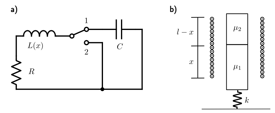
The electronic setup of our kicker boards has already been described in our previous ETDPs [1,37]. The board design is openly available under [38]. We approximate the real electric circuits by the following abstraction shown in fig. 2a).

We use an insulated-gate bipolar transistor (IGBT) to switch the kicker. Assume that the capacitor is initially charged to some voltage U(0). In its onstate the IBGT discharges the capacitor over the solenoid. A resistor is added to model losses inside the solenoid cable. When thge IGBT turns off, the capacitor voltage is no longer applied to the solenoid. The current through the solenoid dies down due to resistive losses. To summarize: depending on whether the IGBT is on or off, we model the electronic part of the kicker as an RL or RLC circuit respectively. The finite switching time of the IGBT is neglected.

The mechanical construction of our kicker modules also has been outlined in our previous (E)TDPs [39, 40]. A plunger consisting of two different materials with relative magnetic permeabilities μ¹ and μ² is placed inside the solenoid like shown in fig. 2b). In our design, the coil is wound around a thin layer of plastic. We denote the cross-sectional area of the plunger with A1, the total cross-sectional area of the solenoid with A and the cross-sectional area of the plastic layer with A² = A−A1. When current passes through the coil, the plunger accelerates forwards, increasing the length x of the material with permeability μ¹ inside the solenoid of length l. Therefore, the inductance L(x) of the solenoid is not constant, but rather depends on the position x of the plunger. A spring with spring constant k is used to pull the plunger back into its original position after the kick.

For now, only consider the case of an conducting IGBT, i.e. the capacitor discharging through the solenoid. We decompose the total Lagrangian of the kicker into two parts

$$\mathcal{L} = \mathcal{L}{el} + \mathcal{L}{mech}, \tag{10}$$

one describes only the electric subsystem whith the charge Q on the capacitor as the only degree of freedom, the other describes the mechanical subsystem, which also has only one degree of freedom with x.

A general method to derive Lagrangians for electric circuits is presented e.g. in [41]. The case of the RLC circuit is fairly simple: the energy stored in the capacitor $\frac{Q^2}{2C}$ is treated as a potential energy, while the energy stored in the magnetic field of the inductor $\frac{1}{2}L\dot{Q}^2$ is regarded as a kinetic energy. The electric Lagrangian therefore becomes

$$\mathcal{L}_{\rm el} = \frac{1}{2}L(x)\dot{Q}^2 - \frac{Q^2}{2C}. \tag{11}$$

We explicitly highlight the x-dependence of the inductance here, since it will be relevant later on. The resistor is only relevant for the dissipation function. Since the dissipated power over the resistor is $UI = RI^2$, the dissipation function is given by

$$\mathcal{D} = \frac{1}{2}R\dot{Q}^2. \tag{12}$$

The mechanical part of the Lagrangian is also very simple. The plunger has a mass m and therefore a kinetic energy $\frac{1}{2}m\dot{x}^2$. We assume for simplicity that at x=0 the spring is at equilibrium. Hence, it stores a potential energy of $\frac{1}{2}kx^2$. We observe that at least for our setup, the spring is weak enough to be safely neglected. We only keep it here for the sake of completeness. The mechanical Lagrangian becomes

$$\mathcal{L}_{\text{mech}} = \frac{1}{2}m\dot{x}^2 - \frac{1}{2}kx^2. \tag{13}$$

Now it only remains to find an explicit formula for L(x). The inductance is defined as the ratio if magnetic flux through the solenoid and the current causing this flux. Unfortunately, neither the plastic layer between plunger and coil, nor finite size effects of the coil are negligible in our setup. The steady-state magnetic field on the symmetry axis of a finite coil of length l with N windings and radius r is given by [42]

$$H(s) = \frac{N}{2l}\dot{Q}\left(\frac{l-s}{\sqrt{r^2 + (l-s)^2}} + \frac{s}{\sqrt{r^2 + s^2}}\right)e_x. \tag{14}$$

For non-circular coils, we replace the radius with an effective radius $r = \sqrt{\frac{A}{\pi}}$. This approximation to the true equivalent radius, i.e. the radius of a circular coil with the same inductance, is within 0.1% for coils with a length of at least half their diameter [43].

Since the characteristic timescale of the kicker is on the order of milliseconds and its spatial extension is a few centimeters, the quasi-static approximation to Maxwell's equations is well justified. This means we can safely neglect effects of electromagnetic radiation and a finite propagation speed of the fields. For more information on quasi-static electromagnetism see e.g. [44].

To simplify the calculations, we assume that this expression is valid everywhere inside the solenoid. This simplification is justified post-hoc by the fact that the resulting inductance matches experimental values quite well. Further, since the tangential component of H across the plunger to plastic interface has to be continuous [45], we use eq. (14) for the core-filled part of the solenoid as well. However, this leads to a problem: it implies that the normal component of B cannot be continuous at the interface between the plunger materials, violating Maxwells equations. This shows that the magnetic field behaves in a more complex manner at the material boundary. However, as this is only a problem directly at the boundary, we neglect this effect for simplicities sake.

The inductance is defined as the proportionality constant between the current and the total flux through the coil. From the expression of the magnetic field, we can calculate the total flux Φtot through the solenoid by computing the flux ΦA(s) = (A² + µr(s)A1)H(s) through every loop and summing the results. Since the exact geometry of the loops is difficult to model, we assume a constant winding density N/l and replace the sum by an integral

$$\Phi_{\text{tot}} = \frac{N}{l} \int_{0}^{l} \Phi_{A}(s) ds = \frac{N}{l} \mu_{0} \int_{0}^{l} (A_{2} + \mu_{r}(s) A_{1}) H(s) ds$$

$$= \mu_{0} \frac{N^{2}}{l^{2}} \dot{Q} \left( \sqrt{r^{2} + l^{2}} \left( A_{2} + \frac{\mu_{1} + \mu_{2}}{2} A_{1} \right) + \frac{1}{2} A_{1} (\mu_{1} - \mu_{2}) \left( \sqrt{r^{2} + x^{2}} - \sqrt{r^{2} + (l - x)^{2}} \right) \right). \tag{15}$$

and can be directly read off from the equation above to be

$$L(x) = \frac{\Phi_{\text{tot}}}{\dot{Q}} = \mu_0 \frac{N^2}{l^2} \left( \sqrt{r^2 + l^2} \left( A_2 + \frac{\mu_1 + \mu_2}{2} A_1 \right) + \frac{1}{2} A_1 (\mu_1 - \mu_2) \left( \sqrt{r^2 + x^2} - \sqrt{r^2 + (l - x)^2} \right) \right). \tag{16}$$

We now have all the necessary ingredients to write down the equations of motion. For convenience of notation, we collect the frequently occuring corrections due to the finite size of the solenoid in the function

$$f_1(x) = \frac{1}{2} \left( \frac{l - x}{\sqrt{r^2 + (l - x)^2}} + \frac{x}{\sqrt{r^2 + x^2}} \right). \tag{17}$$

The Euler-Lagrange equation (9) for the plunger position yields

$$m\ddot{x} + kx - \frac{1}{2}\frac{\partial L}{\partial x}(x)\dot{Q}^2 = 0 \tag{18}$$

where the derivative of the inductance can be computed to be

$$\frac{\partial L}{\partial x}(x) = \mu_0 \frac{N^2}{l^2} A_1(\mu_1 - \mu_2) f_1(x). \tag{19}$$

Inserting this expressions back into eq. (18) reads

$$m\ddot{x} + kx - \frac{1}{2}\mu_0 \frac{N^2}{l^2} A_1(\mu_1 - \mu_2) f_1(x) \dot{Q}^2 = 0. \tag{20}$$

Similarly, for the capacitor charge, the Euler-Lagrange equation (9) becomes

$$L(x)\ddot{Q} + \frac{\partial L}{\partial x}\dot{x}\dot{Q} + R\dot{Q} + \frac{Q}{C} = 0$$

$$\Leftrightarrow L(x)\ddot{Q} + \mu_0 \frac{N^2}{l^2} A_1(\mu_1 - \mu_2) f_1(x)\dot{x}\dot{Q} + R\dot{Q} + \frac{Q}{C} = 0. \tag{21}$$

Unfortunately, due to the $\dot{x}\dot{Q}$ and finite-size terms, the Euler-Lagrange equations are highly nonlinear. We did not find any closed form analytic solutions for these types of equations. Instead, we needed to fall back to solving them numerically with the Runge-Kutta method of fourth order (see e.g. [46]). To do this, we must first convert the second order Euler-Lagrange equations to an equivalent system of first order equations. This is achieved by introducing the velocity v of the plunger and the current I coming from the capacitor. The first order equations of motion then become

$$\dot{x} = v \tag{22}$$

$$\dot{v} = \frac{1}{m} \left( -kx + \frac{1}{2} \mu_0 \frac{N^2}{l^2} A_1(\mu_1 - \mu_2) f_1(x) \dot{Q}^2 \right) \tag{23}$$

$$\dot{Q} = -I \tag{24}$$

$$\dot{I} = \frac{-1}{L(x)} \left( RI - \frac{Q}{C} + \mu_0 \frac{N^2}{l^2} A_1(\mu_1 - \mu_2) f_1(x) vI \right). \tag{25}$$

This procedure can be repeated to obtain the equations of motion after the IGBT cuts the connection to the capacitor

$$\dot{x} = v \tag{26}$$

$$\dot{v} = \frac{1}{m} \left( -kx + \frac{1}{2} \mu_0 \frac{N^2}{l^2} A_1(\mu_1 - \mu_2) f_1(x) I^2 \right) \tag{27}$$

$$\dot{I} = \frac{-1}{L(x)} \left( RI + \mu_0 \frac{N^2}{l^2} A_1(\mu_1 - \mu_2) f_1(x) vI \right). \tag{28}$$

5 Experiments

Now that a model of the kicker has been set up, we need to determine the relevant parameters and validate that it correctly describes the real device. Most of the parameters are either specified by the manufacturer or can be determined by standard methods. Table 1 contains the relevant values for our linear kicking device.

The only parameter missing from this listing is the magnetic permeability μ¹ of back half of the plunger. The magnetic permeability of steel can vary multiple orders of magnitude, depending on the exact mixture and production process of the material. Therefore, we have to come up with some way to measure the permeability of each particular plunger. This was done by fixing the plunger in different positions inside the coil and observing the change of inductance.

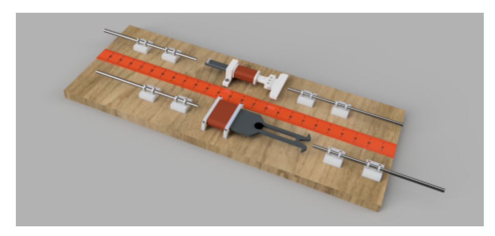
We designed a experiments setup to achieve accurate measurement of the plunger. The windings and the plastic part of the coil are fixed to a wooden base board. The plunger can be moved and adjusted through the coils using two threaded rods – one on each side. A measuring tape glued to the surface gives indicates the current position of plunger.

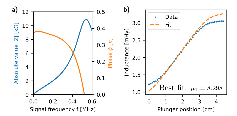
The impedance of the kicker solenoid was measured by a Bode100 device. It generates a Bode plot of the frequency dependent impedance. An ideal inductor has an impedance of Z = i2πfL.

However, any real device suffers from parasitic effects. At low frequencies, the resistance of the wires dominates the impedance, at frequencies higher than the resonance, which we observe at roughly 0.5 MHz (cf. fig. 4), the parasitic capacitance between the coil windings becomes prevalent. A good indicator of the inductively dominated region is that the measured phase ϕ of the complex impedance remains flat at a value close to π/2. Based on this, we evaluate

$$L \approx \frac{|Z(f)|\sin(\phi(f))}{2\pi f} \tag{29}$$

at the frequency f = 15 kHz.

The magnetic permeability μ¹ is then obtained by fitting eq. (16) to the inductance data using the scipy implementation of the trust-region optimization algorithm [47]. The best fit value is obtained as μ¹ = 8.298 ± 0.004. The data is shown in fig. 4.

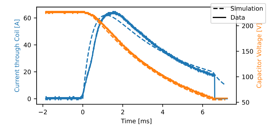
Next, we validate the theoretical kicker model by simulating a full kick and comparing the capacitor voltage, solenoid current and ball velocity to measurements. For details on the measurement of current and voltage, refer to [2]. The outgoing ball velocity was measured with two light barriers. The simulation starts with the plunger at rest at a position of x⁰ = 7 mm. Meaning a small part of the plunger is already inside the coil. The capacitor is discharged over the solenoid for 6.5 ms, which corresponds to the maximal kick power that we use during the game. The equations of motion are solved numerically with the Runge-Kutta method of fourth order [46] and a timestep of Δt = 1 µs. The simulation stops once the plunger reaches x = l, at which point we assume it collides with the ball. From energy- and momentum conservation one can derive the outgoing ball velocity after a fully elastic collision with the plunger to be

$$v_{\text{Ball}} = \frac{2m_{\text{plunger}}v_{\text{plunger}}}{m_{\text{plunger}} + m_{\text{Ball}}}. \tag{30}$$

The final ball speed from the simulation is 6.8 m/s, which is accurate to 1.4% compared to the measured value of 6.9 m/s. The current and voltage profiles also match the measurement well, as can be seen from fig. 5.

Table 1: Values of the model parameters for our linear kicker. The capacitance is given by the vendor, the initial voltage is controlled by our kicker board. The resistance of the solenoid wire can be measured by a multimeter. The coil windings were counted when the solenoid was manufactured. The cross-sectional areas and length were read from the CAD files for the solenoid plastic layer. The front part of the plunger is built from aluminium, the magnetic permeability of which is well-known. The mass of the plunger was measured with a standard kitchen scale. The spring constant was determined by linear regression of the dilation from known weights.

6 Results and discussion

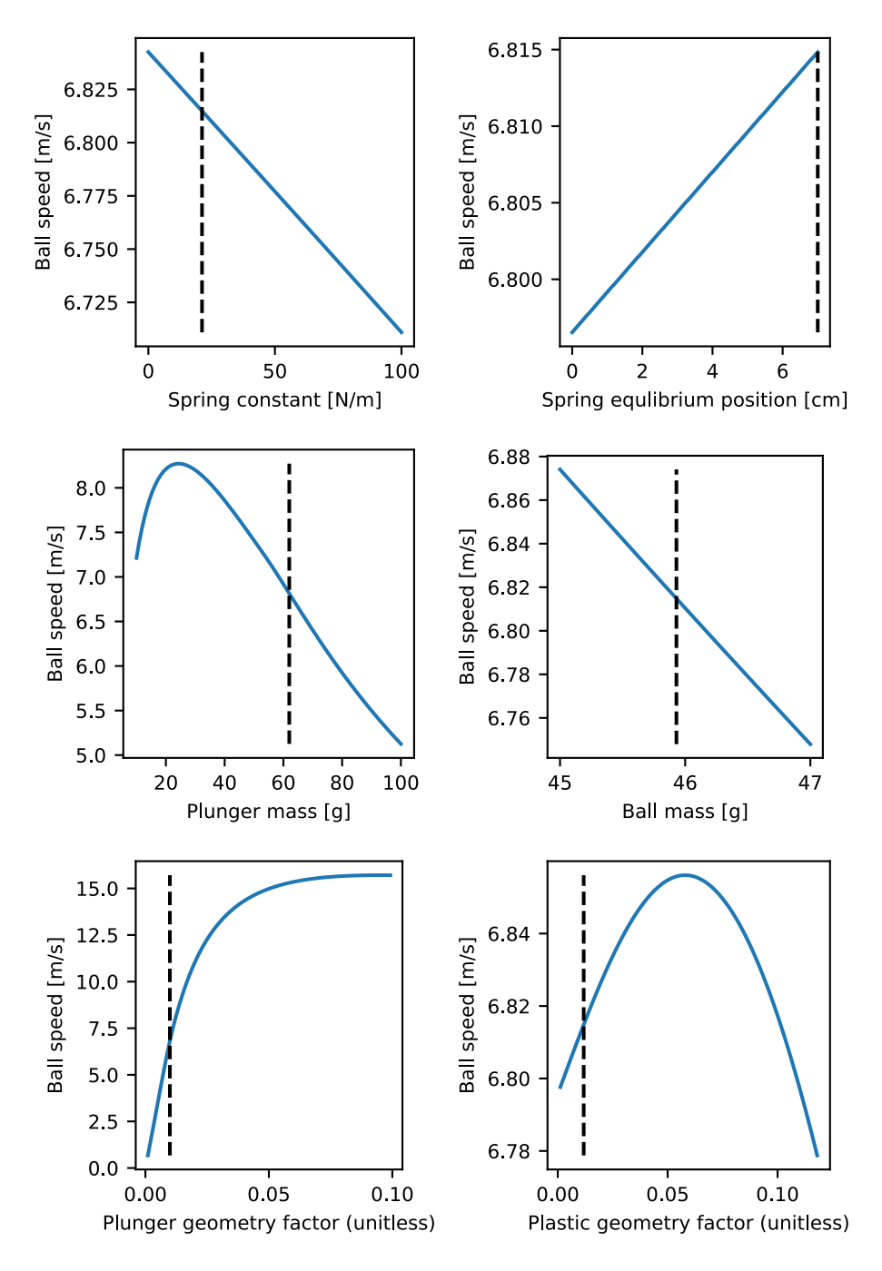
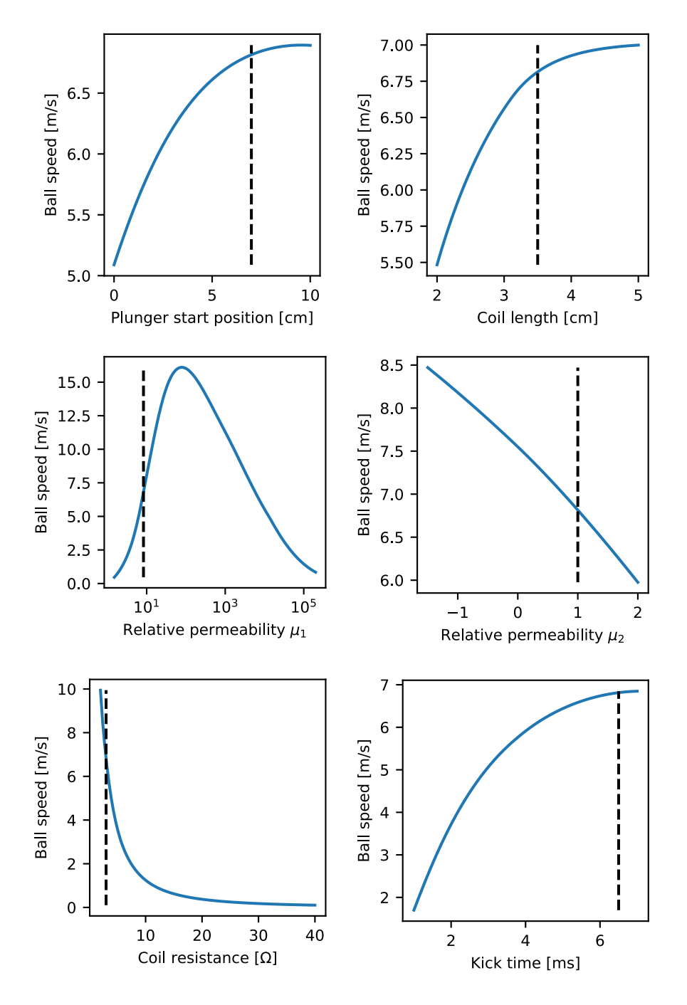
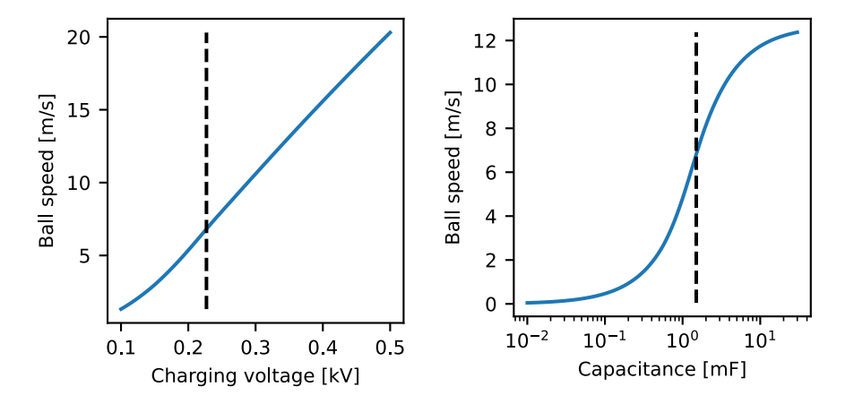
Since the model matches our observations well, we can use it to make predictions on the kick power of different kicker designs. We investigate the influence of the spring constant, its equilibrium position, the plunger and ball mass, the coil geometry, the start position of the plunger and the coil length, the relative permeabilities of the two plunger materials, the resistance, capacitance and charging voltage of the electrical circuit and the total duration at which the IGBT allows the capacitor to discharge over the solenoid on the speed of the ball after a linear kick.

Each parameter was varied in a region, which we deemed possibly realistic, while keeping all the other parameters constant. Note that this does neglect codependence in the parameters, e.g. it is typically not possible to change the magnetic permeability of the plunger without changing its material, which will in turn also affect its mass. Since the parameters describing the geometry of the solenoid, namely l, A and N only enter the equations of motion in the form of the factor $A\frac{N^2}{l^2}$, we only consider the dependence of the kick power on this total factor instead of each of these parameters independently. However, the length of the coil does need an independent consideration nontheless, since it also affects the length the plunger needs to travel in the simulation before it hits the ball.

We want to particularly motivate our choices of ranges for μ₁ and μ₂, since they might be surprising at first glance. We consider values of μ₁ in the range of 1 to 200000, the former representing a completely non-magnetic material and the latter being a typical value for iron. For μ₂ we decided to also consider diamagnetic materials, which would be repelled by the magnetic field and therefore contribute an additional accelerating force to the plunger.

The results are shown in fig. 6, fig. 7 and fig. 8. Whenever the possible range of values comprises more than two orders of magnitude, we opted to scale the x-axis of the plots logarithmically.

There are a few points we want to highlight. First, the nonlinear nature of the equations of motion clearly becomes visible in the results. The kick power either plateaus or exhibits a local optimum for parameters like the plunger mass, coil and plunger geometry, relative permeabilities, and capacitance.

We awant to highlight that the kick power in our current setup would be maximized by a plunger with μ₁ ≈ 100 and decreases for higher values. The explanation for this is that for high values of μ₁ the plunger induces a considerable countervoltage already at slow velocities, inhibiting the capacitor from running current through the solenoid. Other parameters, like the spring constant and equilibrium position, the mass of the ball and the charging voltage show a mostly linear impact on the ball speed in the considered range. The kick power is most sensitive to the plunger cross-section, to μ₁, to the resistance of the coil wire, to the capacitance and to the charging voltage.

7 Summary and outlook

In this paper, we presented a physical model of the inductive kicking mechanism in our robots. The model is based on Lagrangian mechanics, which allows us to derive the equations of motion for both the electrical and mechanical degrees of freedom simultaneously. Further, we describe a method of experimentally determining the magnetic permeability of the magnetic part of the plunger by observing the change of inductance as the plunger is moved through the solenoid. Moreover it was validated that our model matches observations made from the real kicking device. We observe that the behaviour of the kicker is nonlinear, with many parameters showing either saturation or local optima in the kick power.

In the future we want to use the model to aid in our design of the kicker module for the next robot generation. Since the runtime of an individual simulation is on the order of a second, one could for example wrap the simulation in a black-box optimization algorithm to automatically find a set of parameters within given constraints that optimize efficiency or overall power of the kick.

References

1. Bergmann, P., Engelhardt, T., Gareis, E., Hahn, U., Heineken, T., Hopf, V., Möser, R., Mutter, F., Schmid, M., Schmidt, M., Stadler, M., Wendler, A., Wiedmann, M.: ER-Force 2023 Extended Team Description Paper. (2023)
2. Böhm, T., Gareis, E., Hahn, U., Heineken, T., Hopf, V., Schmid, M., Schmidtmeier, C., Wiedmann, M.: ER-Force 2024 Extended Team Description Paper. (2024)
3. Cosenza, C.S., Couto, G.C.K., Germano, L., Correa, L.G., Barreira, L.d.S., de Melo, C., Bozza, M., de Souza, M.P., Silveira, O.C.B., Dias, G.S., Nihari, Y., Rosa, P.F.F.: RoboIME: From the top of Latin America to RoboCup 2018. (2018)
4. Boussicault, A., Felix, P., Hofer, L., Ly, O., N'Guyen, S., Passault, G., Pirrone, A.: AMC – Team Description Paper. (2018)
5. Rodrıguez, S., Rojas, E., Perez, K., Lopez, J., Calderon, J.M.: STOx's 2014 Extended Team Description Paper. (2014)
6. MacDougall, M., Hashemi, A., Lip, O.C., Sousa, C., Whyte, G., Golsteyn, Q., Petzen, R., Deutsch, D.: 2019 Team Description Paper: UBC Thunderbots. (2019)
7. Hirohashi, T., Matsumoto, Y., Tomioka, D., Naito, Y., Mitsuishi, K., Obara, T., Mitsushima, A., Murai, R., Okunishi, S., Ochiishi, K., Otake, S., Katsumi, B.: RoboCup 2024 TEAM DESCRIPTION PAPER Ri-one. (2024)
8. Allali, J., Bezamat, J., Boussicault, A., Denieport, R., Felix, P., Ly, O., N'Guyen, S., Mignot, V., Passault, G., Saliba, T.: NAMeC - Team Description Paper Small Size League RoboCup 2019 Application of Qualification in Division B. (2019)
9. Almagro, J., Feltracco, J., Medrano, R., Naeem, S., Neiger, J., Osawa, R., Peterson, E., Shaw, A., Woodward, M.: RoboJackets 2018 Team Description Paper. (2018)
10. Angelo Gurzoni Jr., J., Francischini, G., Malheiro, D., Cortez, M., Camargo, F., Fill, F., Felizatti, R.L., Bellatrix, P., Bianchi, R.A.C., Tonidandel, F.: RoboFEI 2011 Team Description Paper. (2011)
11. Panyapiang, T., Thanomyart, R., Sukvichai, K.: Skuba 2013 Extended Team Description. (2013)
12. Seegemann, L., Zeug, F., Ebbighausen, P., Waldhoff, L., Westermann, M., Knackstedt, S., Känner, M., Füchsel, T., Hart, R., Pahl, T.: luhbots Soccer Team Description for RoboCup 2023. (2023)
13. Morales, M., Possani, A., Garza, A.C., Cordova, A., Arrieta, A.E., Sosa, J.C.G., Estrada, E.P., Renterıa, J.P., Rodrıguez, K.L.P., Galeana, H.R., Brena, J.S., Teran, F., Reyesvera, U.: Eagle Knights 2013: Small Size League Team Description Paper. (2013)
14. Zickler, S., Bruce, J., Biswas, J., Licitra, M., Veloso, M.: CMDragons 2009 Extended Team Description. (2009)
15. Takata, S., Horie, Y., Aoki, S., Fujiwara, K., Degawa, T.: MCT Susanoo Logics 2014 Team Description. (2014)
16. Develer, U., Oksuz, H.Y., Turan, G., Akar, M.: BRocks 2016 Team Description. (2016)
17. Ahumada, G., Arriagada, S., Banda, C., Barrientos, C., Callejas, E., Carrasco, C., Jara, M., Nettle, C., Riquelme, P., Rodenas, T., Solis, M., Suarez, M.: IRSS Deluxe Team Description Paper. (2014)
18. Anschuetz, E., Cruz, J., Donahue, K., Schumann, S., Zigmond, E.: 2016 RFC Cambridge Team Description Paper. (2016)
19. Bouchard, S., Lachapelle, F., Lebel, P., Verret, B.: ULtron 2018 Team Description Paper. (2018)
20. Poorjandaghi, S.S., Monajjemi, V., Mehrabi, V., Nabi, M., Koochakzadeh, A., Atashzar, S.F., Omidi, E., Sheikhi, E., Bahmand, A., Pour, S.M.M., Saeidi, A., Shamipour, S., Karkon, R.: Parsian (Amirkabir Univ. Of Technology Robocup Small Size Team) Team Description for Robocup 2011. (2011)
21. Horii, T., Sato, R., Hattori, H., Iwauchi, Y., Mizutani, S., Zenji, S., Baba, K., Inukai, K., Inagaki, K., Kanei, H., Goto, R., Asakura, T., Watanabe, M., Ito, K., Sugiura, T.: KIKS 2010 Extended Team Description. (2010)
22. Gaurav, A., Jasoria, T., Panda, S.K., Dalal, P., Mittal, H., Sinha, S., Agarwal, S., Kumar, R., Kumar, R., Ramnani, P., Reddy, K.S., Bhat, M., Raj, V., Aggarwal, S., Kirtania, A., Chilukuri, G.R., Kartik, M., Agrawal, A., Roy, A., Praharaj, A., Jerry, J., Dwivedi, A., Surya, D.P., Mondal, R., Garg, C., Gupta, A., Sharma, S., Bhushan, M., Sharma, S., Roy, A.: KgpKubs 2019 Team Description Paper. (2019)
23. Leon, J.M.D., Tan, M., Piel, J., Oh, H., Woldeghebriel, E., Gonzalez, R., Sales, P., Heinle, D., Samayoa, J., Badgett, M., Lee, N., Liu, R., Cheung, R., Perez, I., Gupte, A., Weber, D., Iqbal, B., Hamad, N., Fong, A., Pho, K.: MIT RoboTeam 2020 Team Description Paper. (2020)
24. Srikluan, M., Srithong, A., Prisuwun, S., Paocharoen, J., Chaiburee, W., Karnjanadecha, M.: Khainui Team Description for Robocup 2010. (2010)
25. Alaei, S.A., Abdi, M., Hajihoseini, A., Ghadimi, H., Abbasi, D., Sarbandi, M., Khandani, M.M., Sayardust, S., Keshavarzi, S., Najafi, M., Hosseinzadeh, M., Manuchehri, M.S., Kiaei, A., Abdolghafar, M., Forouzideh, A., Alikhani, S., Darestani, E., Nasiri, S.M.: OMID 2011 Team Description. (2011)
26. Veeraghanta, A., Bryant, H., Zheng, S., MacDougall, M., Guido, S., Bontkes, L.: 2024 Team Description Paper: The Bots. (2024)
27. ABIYEV, R.H., GUNSEL, I., AKKAYA, N., AYTAC, E., ARSLAN, M., EMREM, F., SAY, G., CAGMAN, A., KORKMAZ, S., DAGLI, I., ARICI, M.: NEUIslanders 2014 Team Description Paper. (2014)
28. Croll, E., Freije, R., de Haan, K., Okken, B., Plompen, R., Rubbens, B., Timmer, R., Tolboom, S., de Weerdt, D., Weijers, I., Westra, W.: RoboTeam Twente 2017 Team Description Paper. (2017)
29. Ryll, A., Jut, S.: TIGERs Mannheim (Team Interacting and Game Evolving Robots) Extended Team Description for RoboCup 2020. (2020)
30. Liu, Y.: Botnia Dragon Knights - Team Description Paper for RoboCup 2010 Small Size League. (2010)
31. Blank, P., Bleier, M., Dexler, S., Kallwies, J., Kugler, P., Nordhus, P., Tully, J.: ER-Force Team Description Paper for RoboCup 2008. (2008)
32. Broaddus, P., Johnson, B., Jun, B., Maheshwari, R.: Stanford Robotics Club 2014 Team Description. (2014)
33. Barcelos, A.O.P., Segre, J.L.L., de Lima, L.O., Gemignani, R., Bramigk, V., Rosa, P.F.F.: RoboIME: on the road to RoboCup 2014. (2014)
34. Wasuntapichaikul, P.: Skuba 2010 Extended Team Description. (2010)
35. Palmer, A., Head, C., Lai, M., Poon, H., Lin, T., Wong, A., Wang, B., Fraser, J., Yu, K., Wang, B., Villar, C., Lum, S., Kalla, T., Gabaldon, A., Lam, A., Holdjik, S., Tai, W., Su, W.Y., Lee, B., Wu, C., Nino, D., Peri, K., Yoon, R., Jang, E., Wong, P., Cho, B., Tang, R., Leson, A.: 2013 Team Description Paper: UBC Thunderbots. (2013)
36. Goldstein, H., Poole, C.P., Safko, J.: Classical Mechanics. Third edition edn. Addison-Wesley (2001)
37. Bergmann, P., Engelhardt, T., Heineken, T., Hopf, V., Schmid, M., Schmidt, M., Schofer, F., Schuh, K., Stadler, M.: ER-Force 2022 Extended Team Description Paper. (2022)
38. Robotics Erlangen e.V.: Open Source SSL Robot Hardware. https://github.com/robotics-erlangen/hardware Accessed: 2025-01-05.
39. Bayerlein, H., Danzer, A., Eischer, M., Hauck, A., Hoffmann, M., Kallwies, P., Lieret, M.: ER-Force Team Description Paper for RoboCup 2014. (2014)
40. Bühlmeyer, J., Burk, D., Danzer, A., Kronberger, S., Lobmeier, C., Niebisch, M., Eskofier, B.M.: ER-Force Extended Team Description Paper RoboCup 2017. (2017)
41. Scherpen, J.M.A., Jeltsema, D., Klaassens, J.B.: Lagrangian modeling of switching electrical networks. Systems & Control Letters 48(5) (April 2003) 365–374
42. Callaghan, E.E., Maslen, S.H.: The Magnetic Field of a Finite Solenoid. Technical Report NASA-TN-D-465 (October 1960) NTRS Author Affiliations: NASA Lewis Research Center NTRS Document ID: 19980227402 NTRS Research Center: Legacy CDMS (CDMS).
43. Grover, F.W.: Inductance Calculations: Working Formulas and Tables. Special edition prepared for instrument society of america edn. Dover Publications (1973)
44. Larsson, J.: Electromagnetics from a quasistatic perspective. American Journal of Physics 75(3) (March 2007) 230–239
45. Griffiths, D.J.: Introduction to Electrodynamics. 3rd ed. edn. Prentice-Hall, Inc., New Jersey (1999)
46. Butcher, J.C.: Numerical methods for ordinary differential equations. 2. ed. edn. Wiley, Chicester (2008)
47. Branch, M.A., Coleman, T.F., Li, Y.: A subspace, interior, and conjugate gradient method for large-scale bound-constrained minimization problems. SIAM Journal on Scientific Computing 21(1) (1999) 1–23