KIKS Extended Team Description for RoboCup 2025
Mizuki Nonoyama, Haru Niimi, Takahiro Miyauchi, Yota Dori, Chihiro Takanashi, Ryuto Tanaka, Chiaki Naito, Kazuaki Harada, Hirokazu Komatsu, Dai Oikawa, Toko Sugiura
Nat'l Inst. of Tech., Toyota College, 2-1 Eisei-cho, Toyota, Aichi 471-8525, Japan; Kindai University, 1 Takayaumenobe, Higashihiroshima, Hiroshima 739-2116, Japan
https://www.ee.toyota-ct.ac.jp/staff/sugi/RoboCup.html
Abstract This paper describes the current situation of the system development of the KIKS team in order to qualify for the RoboCup 2025. In particular, the development of active markers for demonstration use, the contents related to path planning for obstacle avoidance and a discussion of the competitive strength for each team participating in RoboCup world competition are described.
1 Introduction
Team KIKS has continued its year-by-year efforts toward higher-performance hardware and smarter AI system development. In this year, we mainly studied the development of active markers, improvement of pathfinding methods, and analysis of the competitive strength for each team. The details of the experiments are described in each section.
2 Implementation of Active Markers
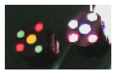
This section describes the studies performed after the RoboCup 2024 regarding the implementation of active markers. During SSL games, the colors of the markers viewed from the camera may be different from those set in SSL-Vision [1] due to changes in the surrounding brightness of the competition field. In addition, we demonstrate SSL robots at many events, some of which are performed under poor conditions, such as direct sunlight or shadows of people or objects on the field, as shown in Fig.1. Under such conditions, the position coordinates of the robots and the ball cannot be obtained successfully. That is, it causes a Vision-Problem, and the smooth progress of the game may be interrupted by the time and required expertise to solve the Vision-Problem. Therefore, we have tried to develop a prototype marker (hereafter described as active marker using full-color LEDs that can be illuminated with a constant color as viewed from the camera, regardless of the surrounding environment. This system is not directly applicable to SSL robots by rules[2], we would like to present it here as a reference.
2.1 Hardware Configuration
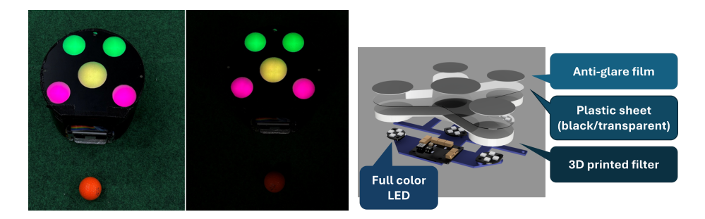
Actual active marker images as seen from the camera with the room light on and off are shown in Fig.2. It shows that the marker can be clearly recognized even in dark conditions. Figure 3 shows an overview of the hardware configuration. Light generated by a full-color LED (NeoPixel: SK6805 built-in) is scattered by passing it through multiple filters made of various materials to improve recognition performance as a marker. The LEDs are controlled by an STM32 microcontroller. LED control commands are received via UART communication connected to the Jetson Nano, which is the robot's main computer. Various sensors can also be attached via I2C communication. The 3D printed filter (made of transparent PETG) shown in Fig.3 is used to scatter the light generated by the full-color LED. If the scattering of light is insufficient, the center of the marker will be white, making it unsuitable for use as a marker. In order to investigate the effect of differences in the infill (internal structure filled with modeling material) on the intensity of scattered light, we compared the homogeneity of light intensity in images viewed from the camera by changing the density and thickness of the infill. The results are shown in Table 1.
Table 1 indicates that at low density (30%), the center is lighter and the periphery is darker. And as the density and thickness increased, the homogeneity was shown to enhance. Within the range of this experiment, the scattered light intensity was almost the same for infill densities and thicknesses greater than 55% and 7.5 mm, respectively. Therefore, a density of 55% and a thickness of 7.5 mm were used in this experiment.
Comparison of scattered light intensity for different infills.
| Thickness[mm] | 30 | 55 | 80 |
|---|---|---|---|
| 2.4 | |||
| 4.8 | |||
| 7.5 | |||
| 10 |
2.2 Block Diagram and the Color Calibration Flow on System
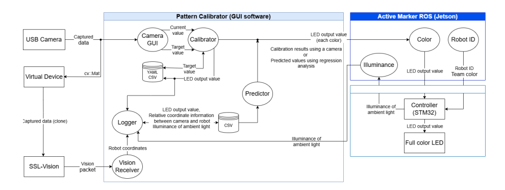
Figure 4 shows a block diagram of the system including the GUI software for active marker color calibration developed in this experiment. In this system, ROS2 (Robot Operating System 2), which is used by many RoboCup teams for robot control, was used to reduce the efforts involved in system installation. The flow of active marker color calibration is described in (1) to (5) below.
- (1) Obtain color information (RGB, YUV) of the active marker from the camera image (assumed to be the current value)
- (2) Calculate the voltage given to the LEDs so that the recorded target value and the current value are matched (refer to the Y value (luminance) for compensation, and refer to the R, G, and B values for color calibration).
- (3) Transmit voltage values to Jetson Nano via ROS2 Topic
- (4) Transmit voltage values to control circuit via UART
- (5) Output to full-color LED
The only preparation for calibration is to set the color of the marker as the target value. Calibration can be performed by clicking color markers in the camera image on the GUI. Therefore, once a color that can be recognized on SSL-Vision is set as the target value beforehand, it can be immediately calibrated even if the marker's color changes during the game.
2.3 Verification of the Responsibility for Changes in Illuminance Around the Field
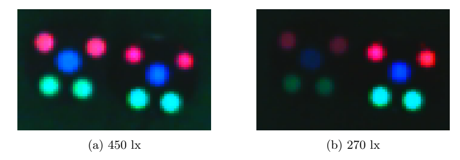
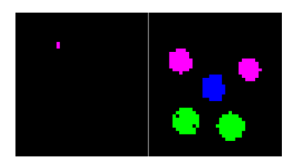
First, in SSL-Vision, thresholds were set for each color to be recognizable in a normal environment (about 450 lx). Next, the active markers were calibrated by changing the ambient light illuminance from 248 to 660 lx (from room lights partially turned off to direct sunlight). Figure 5 shows the influence of ambient light Illuminance on marker color viewed from the camera. Markers made of colored paper became dark at 270 lx and could not be recognized by SSL-Vision. On the other hand, the active markers were automatically calibrated to generate colors that were recognizable as markers under both conditions. Figure 6 shows an example image of marker recognition on SSL-Vision at an illuminance of 270 lx, where colored paper markers could not be recognized. In fact, the colored paper markers were hardly recognized, while the active markers were recognized well. These results indicate that the active markers are appropriately calibrated and can be tuned to the recognizable marker color on SSL-Vision within the illuminance range of this experiment.
2.4 Determination of LED Control Equation with SSL-Vision
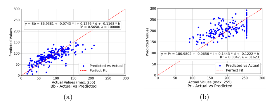
LED light is directional, so the appropriate control value may vary depending on the distance and angle from the camera, even if the ambient light illuminance is the same. Therefore, we tried to find a control equation to automatically control the illuminance of full-color LEDs during a demonstration. First, the color information of each colored paper marker in an environment with an illuminance of 660 lux was obtained as the target value of the active marker. Then, the color thresholds were set on SSL-Vision. Next, the active markers were calibrated by changing the coordinates of the robot on the field, the ambient light intensity, and the height of the camera, while keeping the various camera parameters of SSL-Vision fixed. From the various parameters including the recorded control values, control equations were calculated using the Ridge multiple regression model. The blue component of the blue marker, the red and green components of the yellow marker, the red and blue components of the pink marker, and the green component of the green marker were analyzed. Figure 7 show the measured and predicted results for (a)blue markers (blue component) and (b)pink markers (red component) as examples. Predicted values are plotted on the vertical axis and measured values on the horizontal axis. The dashed line in the figure is a guide plotting the points where the predicted and measured values are in agreement. Therefore, if both values are on the dashed line, the prediction performance can be said high. In the control equation ( derivation function) shown in the figure, i represents the ambient light illuminance, d is the linear distance between the camera and the marker, and h is the height to the camera. In the control equation (derivation function) shown in the Fig.7, i represents the ambient light illuminance, d is the linear distance between the camera and the marker, and h is the height to the camera. The R2 values, which indicate the effectiveness of the control equation, ranged from 0.38 to 0.57. In particular, the graph in Fig.7(b) shows that the R2 value was the lowest due to the. range of the predicted value from 170 to 290 against the measured value of 255. One reason for this may be that the parameter setting of White-Balance in SSL-Vision was insensitive to the red component. In other words, it is considered that the optimal control value derived from the camera was affected by the saturation at the maximum value of 255.
3 Path Planning Using Graph Search
KIKS team has conventionally used an algorithm named "Human-like" [3] to generate paths for robots. Human-like is a fast path planning algorithm designed for local vision robots, and has features such as easier load adjustment and more natural path generation. On the other hand, it has a weak point that if the robot is surrounded by obstacles between the start and end points of the path, it cannot escape from the obstacles. In this section, we evaluated several path finding methods by converting a continuous space such as an SSL field into a discrete graph space and then applying a search algorithm.
3.1 Creating Graph Space
A graph space is a discrete space where points (nodes) are connected by edges (edges with arrows), and search is performed by navigating through the graph. In this section, we describe the conversion processes from a continuous space to a graph space. Three processes from (A) to (C) are as follows.
- (A) First, for each robot on the field (dynamic obstacles), penalty area, goal, etc. (static obstacles), an obstacle model of a circle, edge or polygon is generated with a margin of the robot's radius. If the obstacles overlap each other, they are merged as one obstacle.
- (B) If no obstacles overlap the starting point, two tangents per obstacle can be drawn from the starting point (ignoring the overlap between tangents and obstacles). These can be obtained simply and analytically from the graphic conditions given in (A). Among those tangents, those that overlap with obstacles are excluded. A new node is defined as a point slightly displaced from the point of contact between the remaining tangent and the obstacle, and a new edge is defined as a line drawn between the new node and the starting point. If the new node is close enough to the other node, it is merged with the other node.
- (C) The graph space is generated by repeating (B) with the node obtained in (B) as the starting point.
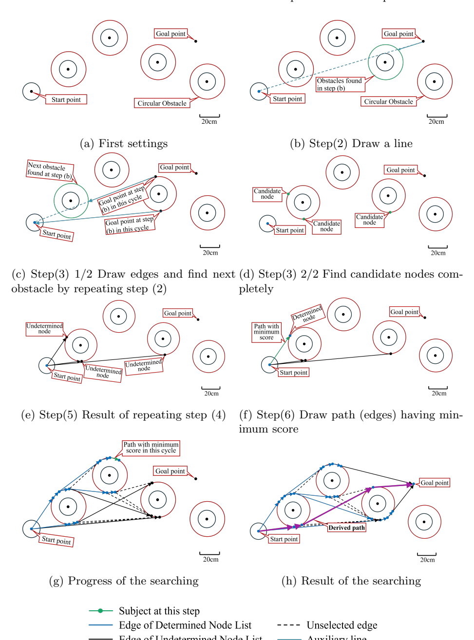
The above process is wasteful in actual search. In fact, the only obstacles to be considered in (B) are those that block them between the starting point and the goal (end point). Also, in case of algorithms that explore from the starting point, even if the initial graph space is incomplete, the graph space is expanded by the necessary amount during the graph search (see § 3.2 for details). Therefore, an efficient graph space will be generated. Next figures 8(a)-(d) partially indicate (A) and (B) in this section.
3.2 Method of Graph Search
For path planning, we mainly used the Dijkstra's algorithm[4], which can take into account the weights of edges. Similarly, we carried out preliminary experiments with the Bellmanford method[5], which can also consider weights, but the number of edges in the graph space in § 3.1 was too large to allow sufficient search at each control cycle, so we do not discuss it in this section.
Algorithms Figures 8(a)-(h) show the process of searching by Dijkstra's method using edge lengths (distances) as weights, and expanding in graph space. Each process is described in detail below. Score of a path is sum of the weights of the edges of the path, and it assumes that there exists at least one path to the endpoint.
Step(1) First, it makes a list to store determined nodes and its path, a list to store undetermined nodes and its path, and a candidate node list. Starting point is stored as an initial value in the determined node list.
- Step(2) The node determined last is denoted as the endpoint. Draw a line from the goal point to the end point and identify the obstacle that will collide with it. The obstacle is used as the starting point in § 3.1 (B) to find the edge in the same way. If no obstacle exists, the endpoint of the search is added to the list of candidate nodes.
- Step(3) If any obstacle exists on the edge, repeat step(2) with the top of the edge as the endpoint until the obstacle is disappeared. If there is no obstacle on the edge, it is added to the next candidate node list (the edge is included in the graph space for search).
- Step(4) Take a node from the candidate node list, and if it is not in the determined node list nor in the path to the endpoint, add the candidate node as a new path to the top of the path to the endpoint. If the candidate node satisfies the condition and is included in the list of undetermined nodes, the scores of the path are compared and the list is updated with the node having a smaller score. On the other hand, if it is not included in the list, it is added to the undetermined node list. The used node is removed from the candidate node list whether it satisfies the condition or not.
- Step(5) Repeat step(4) until the candidate node list is empty.
- Step(6) The node with the smallest path score is taken from the undetermined node list, added to the end of the determined node list, and removed from the undetermined node list. If it is the goal point, the path connected to the node is the answer, and the search is finished.
- Step(7) Repeat steps(2)-(6).
Through the above process, the shortest path is obtained by the Dijkstra's algorithm. In this case, as described in §3.1, the graph space is expanded in steps(2) and (3), and graph search is performed in steps(4)-(6). By repeating these steps, the graph space can be generated to the minimum necessary.
Evaluation We show that the weak points of the Human-like algorithm can be solved by this method. Figures 9a and 9b show the paths generated by the Human-like and Dijkstra algorithms, respectively. In these figures, the yellow robot 0 is at the starting point and the ball is at the goal point. In Fig.9a, the robot is surrounded with obstacles caused by the penalty area and the opponent robot (the path to the goal point is not generated). On the other hand, in Fig.9b, the robot is able to generate a path to the goal point. Table 2 shows the average computation time and standard deviation of the computation time for one search in one game for each method. Table 2 indicates that the Dijkstra's algorithm is sufficient for the control period of 16 ms (60 fps).
Results of computation time for each method
| Type of Method | Average of Computation Time[ms] | Standard Deviation of Computation Time[ms] |
|---|---|---|
| Human-like algorithm | 0.2481 | 0.2408 |
| Dijkstra's algorithm | 0.2897 | 0.5523 |
3.3 Faster Movable Path
In Dijkstra's algorithm, the weight of an edge is generally the length (distance) or cost of the edge. On the other hand, the fastest path to the destination is not necessarily the shortest path. Such situation is especially easy to occur around penalty areas, and the shortest arrival time of a route directly affects the offensive and defensive performance. Therefore, we tried to compare the paths that can arrive at the target point in shorter time (hereinafter denoted as faster movable path) by using the required time calculated by the Eq.(1) as the score of the path (not the weight of edges).
Equation (1) is derived based on the ban-ban control used by KIKS, where $p$ is the position of a node position in the path, $v^0$ is the current speed of the robot, and $\ell^p$ is the extra distance that the robot can move at the end point of each edge when obstacles are taken into account. In Eq.(1), $n$ is defined as $1 \le n \le N$, and $p(N)$ indicates the end point of the path. By the way, the weights of edges in Dijkstra's algorithm must be constant and non-negative regardless of the path. When using Eq.(1), however, it is not constant because it is a function of the edges passed in the past. Therefore, it means that even if the least-cost path is found using Eq.(1) and Dijkstra's algorithm (hereinafter denoted as the timebased Dijkstra's algorithm), it may not always be the fastest path. Therefore, we verify the performance of the time-based Dijkstra's algorithm by comparing with the normal method that takes the shortest distance as the fastest path (hereinafter denoted as the normal Dijkstra's algorithm).
$$\begin{cases} T(n) = \begin{cases} \frac{v_e(n) - v_0(n)}{\alpha_a} & (\ell(n) < \frac{v_m^2(n) - v_0^2(n)}{2\alpha_a}) \ \frac{2\alpha_a \alpha_b \ell(n) + \alpha_b \left(v_m(n) - v_0(n)\right)^2 + \alpha_a \left(v_m(n) - v_e(n)\right)^2}{2\alpha_a \alpha_b v_m(n)} & \text{(otherwize)} \end{cases} \ e(n) = \mathbf{p}(n) - \mathbf{p}(n-1) \ \ell(n) = |\mathbf{e}(n)| \ \cos \theta(n) = \begin{cases} \frac{\mathbf{e}(n) \cdot \mathbf{e}(n-1)}{|\mathbf{e}(n)| |\mathbf{e}(n-1)|} & (n > 1) \ \frac{\mathbf{e}(n) \cdot \mathbf{v}_0}{|\mathbf{e}(n)| |\mathbf{v}0|} & (n = 1) \end{cases} \ v_0(n) = \begin{cases} \cos \theta(n) v_e(n-1) & (n > 1) \ \cos \theta(n) |\mathbf{v}0| & (n = 1) \end{cases} \ v_m(n) = \min \begin{cases} \sqrt{\frac{2\alpha_a \alpha_b \left(\ell(n) + \ell_p(n)\right) + \alpha_b v_0^2(n)}{\alpha_a + \alpha_b}}, v{max} \end{cases} \ v_e(n) = \min \begin{cases} \sqrt{v_0^2(n) + 2\alpha_a \ell(n)}, \sqrt{2\alpha_b \ell_p(n)} \end{cases} \ 0 \le \ell_p(n) \le \min \begin{cases} \frac{v{max}^2}{2\alpha_b}, (\ell(n+1) + \ell_p(n+1)) \cos^2 \theta(n+1) \end{cases} & (n < N) \ \ell_p(n) = 0 & (n = N) \end{cases}$$
Method The robot was run under the same conditions as in an actual game, and the two algorithms were compared for searching from the goalkeeper to the ball. The search was performed every 16 ms, and the predicted arrival time to the target position was calculated from the results. The reason for starting the search from the goalkeeper of the own team is that the search distance is shorter if the ball is in the own team's area and longer if it is in the opponent's area, which includes the predicted situation in a actual game.
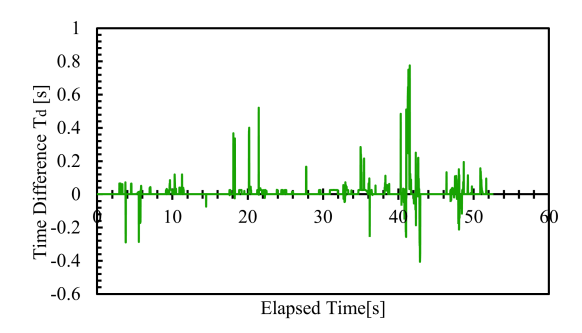
Results The required time for the route by the normal Dijkstra's method and the time-based Dijkstra's algorithm are denoted as $T^n$ and $T^t$, respectively. The time-series dependence of the difference of required times, $T^d = T^n - T^t$, is shown in Fig.10. Figure 10 shows that these differences are positive in many cases. Among the 3151 measured data (for 52.5 sec. of sequence), the positive value was 653 and the negative value was 96. Otherwise, $T^n$ and $T^t$ were the same. On the other hand, a part of $T^d$ is negative, which shows that the timebased Dijkstra's algorithm is not perfect. However, the time-based Dijkstra's method should be used considering that it is at maximum 0.8 seconds faster than the normal Dijkstra method. If the computational resources are sufficient, both methods may be applied in parallel, and the better result may be chosen. The Faster Movable Path generated as described above is expected to play an important role in dominating the game.
3.4 Avoidance
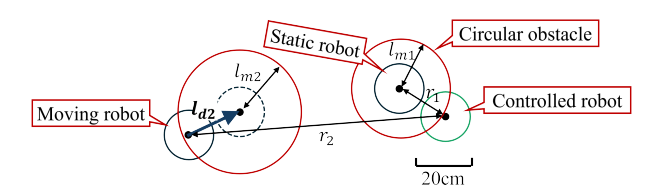
In § 3.1(A), we assumed that the obstacle margin is the radius of the robot, but a dynamic obstacle such as the opponent robot must take into account the amount of movement in time. Therefore, we assume that the dynamic obstacle moves for the time equal to the distance to the target dynamic obstacle divided by the constant velocity. By keeping the margin centered on the predicted moving location and taking into account the acceleration time, it is possible to respond to the rapid movement of the opponent. The margin $l^m$ and the displacement $l^d$ are shown in Eq. (2). Note that the margin of far obstacles is too large in Eq. (2), so the margin is kept constant for obstacles further than a certain distance. In Eq. (2), $r$ is the distance to the dynamic obstacle, $v^r$ is the velocity of the dynamic obstacle, $M^s$ is the margin for static obstacles, and $K_a$, $K_v$, and $K^t$ are constants, respectively. The actual application of eq, (2) is shown in Fig. 11. Even if the actual robot moves along the generated path, it may not be able to avoid obstacles due to external disturbances. When the robot nearly collides with obstacles, it avoids the collision by slowing down, regardless of the path. Then, the robot can arrive at the target position quickly enough by the re-explored path in the next cycle.
$$\begin{cases} \Delta t = \min\left{\frac{r}{K_v}, K_t\right} \ l_m(\Delta t) = M_s + \frac{1}{2}K_\alpha \Delta t^2, \quad \boldsymbol{l_d}(\Delta t) = \Delta t \boldsymbol{v_r} \end{cases}$$
4 Analysis of Team Competitive Strengths
In ETDP2024[6], we analyzed the game log data of all teams participating in the RoboCup 2023 (Div-A) to investigate and analyze the shooting position of the robot that scored, attacking possesion phase, offside line detection, etc. In this year, we will try to analyze the competitive strength of each team. SSL teams use various strategies, but at present, strategies can only be evaluated based on game results, and there is no quantitative evaluation method. Therefore, similar to last year, we try to investigate and consider the competitive strength of each team by analyzing the game logs of RoboCup 2023 and 2024. Based on the results, we aim to find a guideline that will lead to the enhancement of teams' strategies.
4.1 Methods and Procedure
First, we created software to judge and record kicking scenes related to shooting and passing by the robot during a game, and added it on the GUI of KIKS. The recordings include "kicking team", "type of kick", "kick position", "kick direction", "ball arrival point", "goalkeeper position", "time between receiving the ball and shooting", and "number of opponents between the shooter and the goal". Next, we will use machine learning to analyze the kick data of all 44 games in RoboCup 2023 and 2024 (Div-A) to find the expected Goal. Based on these expected values, we will discuss the effectiveness of some team's robot performance and tactics.
Inroducing Expected Goal Expected Goal (xG) is one of the methods used in human soccer recently to express the probability value from 0 to 1 that a shooting will result in a score. The difference between actual goals scored and xG is analyzed and used to improve the efficiency of attacks, evaluation of players and teams, and the choice of shooters.
4.2 Machine Learning Algorithms and Validation Methods
Three models (machine learning algorithms) were used in this section, i.e., Logistic regression[8], Ridge regression[8], and LightGBM classifier[9]. Then, we used two evaluation methods to verify above three models, i.e., ROCAUC score [10] and Cross Val score [11]. The ROC AUC score was verified by the Cross Val score and evaluated by its mean value. The program for data analysis was written in Python. Hyperparameters for each model were adjusted using an optuna[12] based on Bayesian optimization.
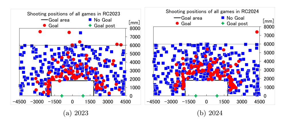
Data Used in the Analysis The training and testing data were shooting data from all games of 2023 and 2024 Div-A shown in Fig.12, respectively. As response variable, we applied the result of shooting (goal=1, other=0( including canceled goals due to foul play)). We used the following explanatory variables.
- (1) Position of the shooter
- (2) Number of opponents between the shooter and the goal
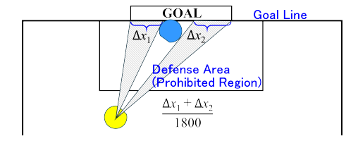
- (3) Scorable goal width(Ratio of shootable width to total goal width when looking at the goal from the attacker's point of view) as shown in Fig.13
- (4) Position of the goalkeeper
- (5) Time between receiving the ball and shooting
4.3 Results and Discussion
Evaluation of the Model The features from (1) to (5) were combined and applied to the model training for 7 patterns (A to F and ALL), and ROCAUC scores were calculated. For (4) and (5) in the previous section, however, there were lacks in log data. One goal in each game in 2023 and 2024 was not available due to blurred vision. Obtained ROCAUC scores are summarized in Table 3. The results in Table 3 indicate that the ROCAUC score is mostly above 0.7 with moderate predictive accuracy.
Verification of three models by ROCAUC score
| Data used in models | Num. of data | Models | | | |
| 2023 | 2024 | Logistic | Ridge | LGBM | |
|---|---|---|---|---|---|
| A{(1)} | 368 | 452 | 0.710 | 0.713 | 0.709 |
| B{(1),(2)} | 368 | 452 | 0.763 | 0.762 | 0.771 |
| C{(1),(3)} | 368 | 452 | 0.757 | 0.756 | 0.717 |
| D{(1),(4)} | 356 | 438 | 0.715 | 0.711 | 0.699 |
| E{(1),(5)} | 356 | 443 | 0.728 | 0.728 | 0.739 |
| F{(1),(2),(3)} | 368 | 452 | 0.766 | 0.763 | 0.740 |
| ALL{(1),(2),(3),(4),(5)} | 355 | 438 | 0.750 | 0.748 | 0.754 |
Evaluation of the Competitive Strength of Each Team Based on the Expected Goal Using the models learned with the 2023 data, we calculated the expected goals for all teams in 2024 and tried to compare them with the goals actually scored. The expected Goal of each model was obtained by ensembling the ROCAUC scores predicted above. Table 4 shows the predictions (xG) obtained using the features of data patterns B, C, and F, which showed the higher predictive performance in Table 3, with the actual scores (Goal). For the most of teams, there is no significant difference between xG and Goal, indicating that they are in god agreemnet. Here, the GOALs in Table 4 for 2024 do not equal the actual goals scored because the goals scored by own-goals were not counted. These results reflect the high probability of actually scoring goals in decisive scenes and situations where it is easy to score. On the other hand, the Immortals had an xG more than three times higher than the actual score, and the large number of shoots suggests that they might have taken a power-play ( aggressive shooting) tactic. This team may increase their score if the performance and control of their robot improves. In contrast, the TIGERs, last year's champions, scored about double the number of actual points than expected Goals. This suggests that the TIGERs have a high competitive ability to score goals in situations that are difficult for other teams to score. Also, since half of the team's shoots were scored, it can be said that the TIGERs are excellent in accurate control of their robots and in judging the scoring scene.
Although the results obtained in these analyses may not directly reflect the current performance of each team, they can be used as a reference for the construction of tactics to increase expected goals.
Expected Goals for the games in 2024
| Team | Rank(2024) | Num. of Shoots | xG(B) | xG(C) | xG(F) | GOALs |
|---|---|---|---|---|---|---|
| TIGERs | 1 | 85 | 22.503 | 21.880 | 21.959 | 45 |
| ZJUNlict | 2 | 142 | 32.190 | 30.923 | 30.472 | 33 |
| ER-Force | 3 | 27 | 6.832 | 6.193 | 6.217 | 6 |
| RobˆoCIn | 4 | 64 | 10.431 | 10.844 | 9.740 | 9 |
| Immortals | 5 | 76 | 14.584 | 14.317 | 13.448 | 4 |
| RoboDragons | 5 | 14 | 2.350 | 2.563 | 2.264 | 1 |
| KIKS | 6 | 16 | 4.782 | 4.528 | 4.811 | 5 |
| Twente | 6 | 18 | 2.752 | 2.784 | 2.425 | 1 |
| luhbots | 6 | 10 | 1.018 | 1.209 | 0.909 | 0 |
Acknowledgments
The authors wish to express their deep appreciation to other KIKS members for the software developments and the hardware manufacturing. This work was supported in part by Grant-in-Aid from JSPS KAKENHI Grant Number 24K06428 and The Sango Foundation for Education in Japan, respectively.
References
- S. Zickler et al., SSL-Vision: The Shared Vision System for the RoboCup Small Size League, RoboCup 2009, LNAI 5949, pp.425-436, 2010.
- Rules of the RoboCup Small Size League, https://robocup-ssl.github.io/ssl-rules/ sslrules.html# vision.
- Jérôme Guzzi et al., Human-friendly robot navigation in dynamic environments, 2013 IEEE Inter. Conf. Robotics and Automation, pp.423-430, 2013.
- E. W. Dijkstra, A note on two problems in connexion with graphs. Numer. Math. 1, pp.269-271, 1959. https://doi.org/10.1007/BF01386390
- Richard Bellman, On A Routing Problem, Quart. Appl. Math. 16, pp.87-90, 1958.
- Ryuto Tanaka et al., KIKS Extended Team Description for RoboCup 2024; https: //ssl.robocup.org/wp-content/uploads/2024/04/2024 ETDP KIKS.pdf
- Sebastian Raschka, Python Machine Learning [in Japanese], impress top gear, 2016.
- sklearn.linear model, https://scikit-learn.org/stable/modules/linear model.html
- lightgbm, https://lightgbm.readthedocs.io/en/stable/
- roc auc score, https://scikit-learn.org/stable/modules/generated/sklearn.metrics. roc_auc_score.html
- cross val score, https://scikit-learn.org/stable/modules/generated/sklearn.model_selection.cross_val_score.html#sklearn.model_selection.cross_val_score
- optuna, https://optuna.org/