SRC Extended Team Description Paper for RoboCup 2025
Yuquan Wang, Fan Yang, Xuanting Liu, Yixuan Wang, Yucheng Gu, Shi Wang, Shenghan Gao, Haohan Zhang, Xiaoxiao Zhu
Student Innovation Center, Shanghai Jiao Tong University, P.R.China
Abstract This paper introduces the achievements which the SRC Team made in the last year. In the software part, we develop the Comprehensive Ball Acquisition Strategy, propose the Best Match for Defence, and also develop a chipping model. In the electronics part, we improve the Power Board and the Electromagnet, and we propose the Adaptive PID method. In the mechanics section, we improve the kicking system and the roller mechanism, and we also conduct dynamic modeling for the robot. We hope to do well in RoboCup 2025 based on these achievements.
Introduction
Software
Comprehensive Ball Acquisition Strategy
The ball acquisition skill integrates multiple ball acquisition methods, including safe ball collection, ball interception, and ball robbing. The core principle of this function is to predict the moments when both the opponent and the robot can reach the ball and determine the optimal ball acquisition method based on the time difference using the model of robot and ball [1]. The function can be called from both the Lua layer and the C++ layer, providing flexibility in its implementation.
The skill provides a function which calculates the ratio of the robot's predicted time to reach the ball to the opponent's predicted time (we define the ratio as emergency index R). This ratio helps determine whether the robot should opt for a safe ball collection or a more aggressive ball interception.
With the ball model, it predicts the ball's position at different time frames. Also, using the robot model, it calculates the time it takes for the robot to reach that point. The function returns the point where the robot can reach the ball before it arrives. This approach ensures that the robot can make the most efficient decision based on real-time predictions.
$$\begin{cases} pos_{ball} = BallModel(\tau) \ t_{me} = MeModel(pos_{ball}) \ t_{he} = HeModel(pos_{ball}) \ R = t_{me}/t_{he} \end{cases}$$
Additionally, the ball fetching skill includes parameters for fine-tuning its performance. The adjust time parameter allows manual adjustment of the robot's ball acquisition time. Setting adjust time to zero relies entirely on the model's predictions, while negative values make the robot's acquisition time faster than the model's predictions.
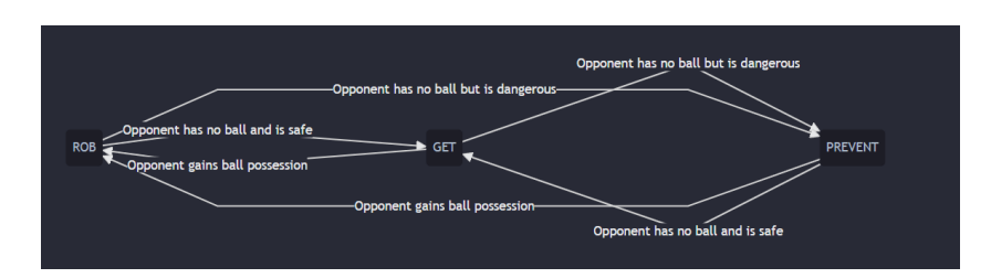
Through the approach explained in Equation (1), the ball acquisition skill could figure out whether it is dangerous right now: we define a constant as a threshold, when R > C it is dangerous. Then it operates within a state machine with three primary states: ROB, PREVENT, and GET. The transitions between these states are based on the game situation and the robot's ability to acquire the ball.
In different state, there are different strategies to fetch the ball:
- ROB: Firstly, the robot attempts to cancel the opponent's obstacle avoidance circle to facilitate ball acquisition. And if the enemy successfully acquires the ball, it must extract the ball from the opponent. By the way, if the opponent is in a shooting position, the robot attempts to block the shot by maneuvering around the opponent.
- PREVENT: The robot blocks the opponent's path to the ball while attempting to acquire the ball at the projected point. Because the interception always occurs when the opponent passes the ball to his teammate, the robot identifies potential receivers of high-speed balls and preemptively blocks their path.
- GET: The robot directly tries to fetch the ball. And when it is close to the target, the robot acquires the ball slowly to prevent pushing it away.
Best Match for Defence
To determine the optimal defensive robot when the ball enters our half of the field, we aim to identify the robot that can reach the ball in the shortest possible time. Traditionally, the strategy has been to assign the robot closest to the ball. However, this approach is not always optimal, as both the robots and the ball possess velocity, and the robots are constrained by their maximum acceleration when changing velocity.
A more effective strategy is to select the robot that minimizes the time required to reach the ball, taking into account the current positions and velocities of both the robots and the ball, as well as the robots' maximum acceleration. This problem can be mathematically formulated as follows: given the current positions of the ball and the robots, their velocities, and the robots' maximum acceleration, determine the robot that can reach the ball in the least amount of time. Solving this requires addressing an optimization problem:
For robot with number i, the relationship between time and position can be expressed as (where ar is the constant standing for maximum acceleration, pr and pb stands for the position of the robot and the ball respectively):
$$p_r^i(t) = p_r^i + v_r^i t + \frac{1}{2} a_r t^2$$
Position of the ball can be expressed as:
$$p_b(t) = p_b + v_b t$$
The interception condition is where the ball and the robot meet:
$$p_r^i(t) = p_b(t)$$
$$\Rightarrow p_r^i + v_r^i t + \frac{1}{2} a_r^i t^2 = p_b + v_b t$$
$$\Rightarrow \frac{1}{2}a_r^i t^2 + (v_r^i - v_b)t + (p_r^i - p_b) = 0$$
Here Equation (6) is a quadratic equation with variable t. In the coding process, we have to figure out how small under the condition that |ar| ≤ amax, the minimized t could be reached.
Electronics
Power Board and Electromagnet
For the purpose of fitting the size of our new mechanics and improving the security of our system, we have made further improvements to the robot's power board and electromagnet, including optimizing the PCB layout, reducing the kicking voltage, and reducing the number of electromagnet turns.
Among the changes, reducing the number of electromagnet turns is a complicated work. The high voltage makes physical experiment quite dangerous, especially when the number of turns of the electromagnet decreases and the discharge current increases, some components will be very easy to damage or even explode. Therefore, a theoretical analysis to determine the number of turns of the electromagnet is more than significant for us.
In previous studies, Song et al. used complex theoretical calculations to study the properties of electromagnets [2]. Yuan et al. used finite element method to simulate the working process of electromagnet [3]. However, the working process of our system is relatively simple, and because of the existence of the ball model, the accuracy requirement is not very strict. Therefore, for theoretical analysis, we use a simple electromagnetic analysis method.
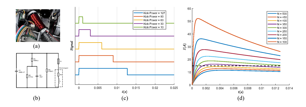
As is shown in Fig. 2(b), we established the circuit model of discharge process according to the circuit design of our power board. The discharge process can be regarded as the zero-input response when the capacitor is fully charged in this circuit model. In the circuit model, the electromagnet is equivalent to a resistor in series with an ideal inductor, where the inductance value L of the inductor and several resistance parameters in the circuit are unknown.
In order to determine the values of unknown parameters in the circuit, we use a combination of theoretical and experimental measurements. According to physical theory, we know that:
$$L \propto N^2$$
where L represents the inductance value of the coil and N represents the number of turns of the coil. Then we measured the inductance value L0 of the old robot's electromagnet with the corresponding first-order circuit, and counted its coil turns N0 by disassembling it. Therefore, the coil inductance of a new electromagnet wound with the same wire diameter and inner barrel can be described as:
$$L = \frac{N^2}{N_0^2} L_0$$
Subsequently, based on the discharge signals of our robot under different kick power, which is shown in Fig. 2(c), the longest discharge time, 12.7ms, was simulated. We simulated the discharge process of the old system, so as to determine some unknown resistance parameters, and then substituted the determined parameters into the circuit model with different turns of electromagnets. The final simulation results are shown in Fig. 2(d). For safety reason, the current should not exceed the black dotted line in the figure. According to the result, our new electromagnet cannot be less than 400 turns. Thus we conducted the experiment using the electromagnet of 300, 350, 400 turns considering the error between theory and practice. And electromagnet was finally determined to be 350 turns after experiment.
Adaptive PID
To improve response speed and reduce overshoot, we implemented an adaptive PID controller using backpropagation on an STM32 microcontroller. This method converts control errors into a loss function and updates parameters via gradient descent. It allows each wheel of the robot to have unique PID parameters, enhancing adaptability to varying conditions and reducing tuning complexity.
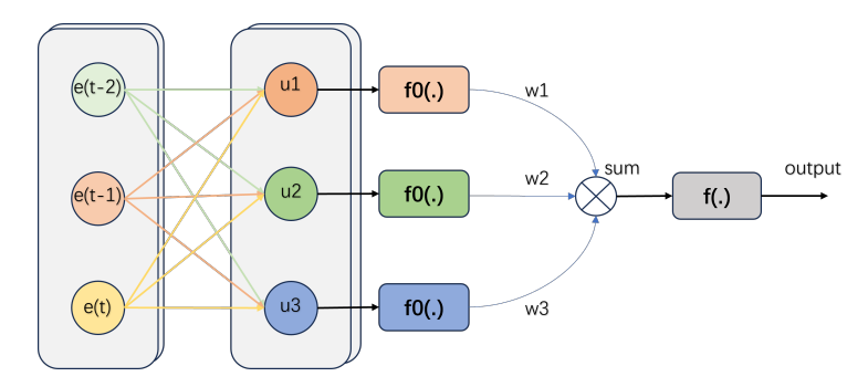
Firstly, based on the structure of the conventional PID controller, we establish a networked controller by defining appropriate connection relationships. The overall architecture of the controller is shown in the figure below. If all connection weights are initialized to 1, and a set of PID parameters is initialized, the controller behaves as a standard incremental PID controller. We replace the three components of the conventional PID controller with three linear functions, denoted as u1, u2, and u3, and introduce nonlinearity through the function f0(.).
Based on the conventional incremental PID controller, we have introduced a nonlinear adjustment element and made the controller parameters variable. The relationship between the error input and the controller output is as follows.
$$\begin{cases} \Delta u = f\left(\sum_{i=1}^{3} u_i\right) \ \nu_i = f_0\left(\alpha_i(t)e(t) + \beta_i(t)e(t-1) + \gamma_i(t)e(t-2)\right) \end{cases}$$
Where ui := ui(t, e(t), e(t−1), e(*t−*2)), and e(t), e(*t−*1), e(*t−*2) represent the error values at the current and the last two sampling instants, respectively.
Considering the actual output requirements of the controller, the final output is subjected to a nonlinear processing function f(·), which is set as output saturation.
To achieve automatic parameter updating, we have designed the following loss function expression. Herein, e(t) represents the difference between the target speed and the actual speed of a single wheel at the current moment, while erot(t) denotes the discrepancy between the speed sent from the host computer and the actual physical speed calculated based on the speeds of the four wheels and the chassis' physical angle at the current moment.
$$e_{total} = \alpha_1 e(t) + \alpha_2 e_{rot}(t)$$
After defining the forward and loss functions, we use backpropagation to update controller parameters. To address gradient vanishing from the final saturation stage, we add a proportional term to penalize larger deviations. The formula is as follows, where output is the controller output and limit is the maximum allowable output:
$$K = \frac{|output|}{limit}$$
Finally, we derive the backpropagation relationships through successive differencing and partial differentiation, thereby achieving automatic parameter updates.
Mechanics
Previously, we have been keeping modifying our structure that is relatively fixed since 2017, however, this year we will be revamping the robot as a whole.
Kick System
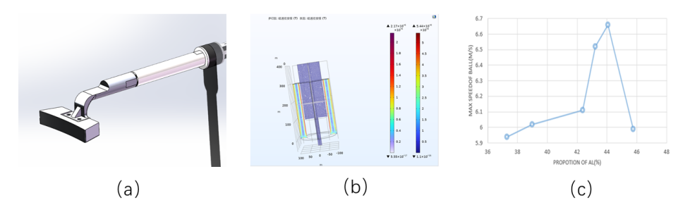
The first noteworthy adjustment involves the kick system. We reduced the number of coil turns from 500 to 350 with the aim of space-saving, as mentioned before. Because of the reduction of the coil turns numbers, we discovered the current also decreased, which would lead to a powerless kick system. Therefore, we changed the proportion of iron and aluminium on the armature of electromagnets and the structure of the electromagnets to make sure the kicking strength is still powerful. However, how much the proportion of iron and aluminum is most appropriate has kept being unsolved. Fortunately, Lu's work has solved the theoretically difficulty [4], our research is based on their conclusion to do some simulation and experiment.
Although, there is a discrepancy between the algorithm and reality, the general trend is basically the same. Based on these graphs, we can tell that as the proportion of aluminium increases, the max speed of the ball increases first and then drops. So we can come to the conclusion that the best proportion of aluminium is about 45%.
However, there are still some problems to be solved. The most serious problem lies in that since our armature is cylindrical, the whole device has two degrees of freedom, which could result in rotation around the axis, we have noticed that many top teams have changed their armature's shape into square, so our ongoing effort is focused on the shape of the armature.
Roller Modifications
To enhance the ball - picking performance of the roller, we first need to analyze the force conditions when the ball comes into contact with the roller. According to the existing Hertzian contact theory, the stress formulas for contact between two spheres and between two cylinders are as follows. Equation (12) represents the contact stress between two spheres, and Equation (13) represents the contact stress between two cylinders.
$$\sigma_{\text{Hmax}} = \frac{1}{\pi} \sqrt[3]{6F \left( \frac{\frac{1}{\rho_1} + \frac{1}{\rho_2}}{\frac{1-\mu_1^2}{E_1} + \frac{1-\mu_2^2}{E_2}} \right)^2}$$
$$\sigma_{\text{Hmax}} = \sqrt{\frac{F}{\pi b} \left( \frac{\frac{1}{\rho_1} + \frac{1}{\rho_2}}{\frac{1-\mu_1^2}{E_1} + \frac{1-\mu_2^2}{E_2}} \right)}$$
In Equation (12) and Equation (13), F represents the externally applied normal force, $\rho_1$ and $\rho_2$ represent the radii of curvature of the two elastic bodies, $\mu_1$ and $\mu_2$ represent the Poisson's ratios of the two contacting materials, and $E_1$ and $E_2$ represent the Young's moduli of the two contacting materials respectively.
However, the actual situation involves the contact between a sphere (golf ball) and a cylinder (roller). Since the contact between spheres is a point contact and the contact between cylinders is a line contact, and considering that the radius of curvature along the axis of the cylinder is infinite, it is not possible to simply modify the above formulas. Instead, they can only be used for estimation purposes. Since the relationship between Young's modulus, shear modulus, and Poisson's ratio is given by
$$G = \frac{E}{2(1+\mu)}$$
and upon reviewing relevant materials, we have obtained the property parameters of materials as shown in Table 1. Furthermore, we have
$$F \ge G_{\text{Golf Ball}}$$
Using the data above, we calculate that $\sigma_{\rm Hmax} \geq 2.3 \times 10^5 \text{ N/m}^2$ . This indicates that at the instant of contact between the ball and the roller, the stress at the contact surface is relatively high. However, due to the extremely short duration of this stress, from a macro perspective, the ball will slightly rebound and then, due to the frictional torque applied by the roller, rotate back under the roller. In actual competitions, when the ball approaches the roller head-on at a high speed, F is relatively large, causing the ball to inevitably rebound. Improvements can be made by reducing the ball's speed to decrease F, or by optimizing the roller's ball-picking structure and the timing of the ball pick-up to provide a greater frictional torque.
The Property Parameters of Materials
| ρ | E | μ | b | |
|---|---|---|---|---|
| Golf Ball | 21.31 mm | 3.0 GPa | 0.38 | 65.16 mm |
| Roller | 5 mm | 2.2 MPa | 0.72 | / |
Robot Kinematics Modeling and Trajectory Prediction
Inverse kinematics of Mecanum wheels converts the robot's desired motion (speed and direction) into wheel rotation speeds, enabling precise and flexible movement. However, uncertainties remain due to differences in environment, robot design, and wheel setup. Forward kinematics is needed to predict the robot's actual path. This section focuses on providing inverse kinematics modeling to control wheel speeds and enabling trajectory prediction to help with debugging and improving motion accuracy.
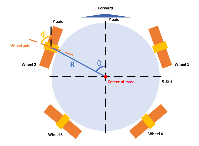
The robot is a cylinder driven by four Mecanum wheels, each with a hub and rollers. Due to size and operability needs, the wheels are unevenly spaced, and their axes do not pass through the robot's center of mass. The robot is also asymmetrical, with its center of mass offset from its geometric center, adding complexity to inverse kinematics modeling.
The geometric dimensions and motion parameters of the robot are described in the following table:
The unit vector in the forward direction of the robot is defined as dfront = [0, 1]. The distance Ri and angle θi between the center of each wheel and the center of mass are calculated as follows:
$$R_i = \sqrt{(x_m - x_c)^2 + (y_m - y_c)^2}$$
$$\theta_i = -\arccos\left(\frac{(x_m - x_c, y_m - y_c) \cdot \mathbf{d}_{\text{front}}}{R_i}\right)$$
The motion state matrix of wheel $i\begin{bmatrix} u_i \ v_i \ w_i \end{bmatrix}$ satisfies:
$$\begin{bmatrix} u_i \ v_i \ w_i \end{bmatrix} = \begin{bmatrix} 1 & 0 & R_i \cos(\theta_i) \ 0 & 1 & R_i \sin(\theta_i) \ 0 & 0 & 1 \end{bmatrix} \begin{bmatrix} u \ v \ w \end{bmatrix}$$
The rotational speed $n_i$ of wheel i can be expressed as:
$$n_i = \frac{60}{2\pi r_i} \left[ \sin(\phi_i) \cos(\phi_i) \ 0 \right] \begin{bmatrix} u_i \ v_i \ w_i \end{bmatrix}$$
The kinematics conversion matrix $A_i$ for a single wheel is defined as:
$$A_{i} = \frac{60}{2\pi r_{i}} \left[ \sin(\phi_{i}) \cos(\phi_{i}) \ 0 \right] \begin{bmatrix} 1 \ 0 \ R_{i} \cos(\theta_{i}) \ 0 \ 1 \ R_{i} \sin(\theta_{i}) \ 0 \ 0 \end{bmatrix}$$
For four wheels, the overall kinematics conversion matrix A is:
$$A = \begin{bmatrix} A_1 \ A_2 \ A_3 \ A_4 \end{bmatrix}$$
Therefore:
$$\begin{bmatrix} n_1 \ n_2 \ n_3 \ n_4 \end{bmatrix} = A \begin{bmatrix} u \ v \ w \end{bmatrix}$$
Now giving the robot forward kinematics modeling:
$$\begin{bmatrix} u \ v \ w \end{bmatrix} = A^{-1} \begin{bmatrix} n_1 \ n_2 \ n_3 \ n_4 \end{bmatrix}$$
However, the matrix A is not invertible. Therefore, we use the pseudoinverse B of the matrix:
$$B = (A^T \cdot A)^{-1} \cdot A^T$$
Thus:
$$\begin{bmatrix} u \ v \ w \end{bmatrix} = B \begin{bmatrix} n_1 \ n_2 \ n_3 \ n_4 \end{bmatrix}$$
With this approach, we can calculate the robot's motion state from the rotational speeds of the wheels. By integrating the velocities, we can obtain the robot's trajectory.
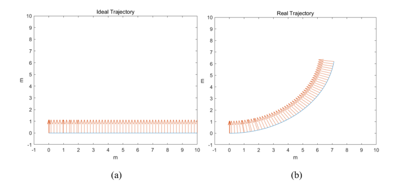
For example, if the robot moves to the right at a speed of 1 m/s, the ideal situation assumes that the front and rear wheels are of equal size. However, in the actual case, the rear wheels have a radius 1 mm larger than the front wheels. The ideal and predicted motion trajectories are shown in the following figures:
In summary, the model predicts the robot's motion trajectory and aids in calibrating its movement in various environments. It can be compared with the actual trajectory measured by the gyroscope to identify deviations caused by factors like uneven ground, wheel slippage, or inaccurate assumptions. Integrating techniques like Kalman filtering reduces sensor noise and uncertainties, significantly enhancing control precision. This improves the robot's adaptability and reliability in complex environments and supports path planning for efficient and accurate movement.
Geometric Dimensions and Motion Parameters of the Robot
| Symbol | Description |
|---|---|
| $[x_c, y_c]$ | Geometric center coordinate of the robot |
| $[x_m, y_m]$ | Mass center coordinate of the robot |
| $[x_i,y_i]$ | Coordinates of wheel $i$ ($i = 1, 2, 3, 4$) |
| $\phi_i$ | Angle between wheel $i$ and the forward direction ($i = 1, 2, 3, 4$) |
| $r_i$ | Radius of wheel $i$ ($i = 1, 2, 3, 4$) |
| $u$ | X-axis translational velocity of the robot |
| $v$ | Y-axis translational velocity of the robot |
| $w$ | Rotation angular velocity around the Z-axis of the robot |
| $n_i$ | Rotational speed of wheel $i$ ($i = 1, 2, 3, 4$) |
Conclusion
In the previous sections, we have detailed our development efforts in the software, electronics, and mechanics sections. In the software section, we introduced the Comprehensive Ball Acquisition Strategy, the Best Match for Defence, and the chipping model. In the electronics section, we highlighted the improvements to the Power Board and the Electromagnet, as well as the proposal of the Adaptive PID method. In the mechanics section, we focused on enhancing the kicking system and the roller mechanism, and conducted dynamic modeling for the robot. Based on these achievements, we are confident that our robots will perform well in RoboCup 2025.
References
- Ziming Chen, Shaoming Pan, Yuquan Wang, Liangcheng Jiang, Yun Bao, Juntong Peng, Yuhong Tan, Xiaoxiao Zhu, SRC Extended Team Description Paper for Robocup 2024. 2024
- Song Y, Shi G, Gu C, Cao Z, Ba K, Hao Y, Kong X. An Improved Method for Calculating the Power Consumption of Electromagnet Coil. Machines. 2024; 12(9):602.
- Xian-ju Yuan, Hong-tao Ling, Tian-yu Qiu, Ji-wei Zhou, Ri-cheng Zhao. Optimization for a Proportional Electro-magnet with High Accuracy Utilizing Finite Element Method. International Journal of Applied Electromagnetics and Mechanics. 2021:267 – 280.
- Lu MengKun, ZhangJunhong, Yi Xianglie, et al. Numerical algorithm of electromagnetic force of cylindrical push-pull electromagnet. Science Technology and Engineering. 2023; 23(30):12958-12965.