Tech United Eindhoven RoboCup Adult Size Humanoid Team Description 2012
P.W.M. van Zutven, S.J. van Dalen, T.M. Assman, J. Caarls, C. Çilli, M.A.P. Aarts, T.P.M. Boshoven, P. Mironchyk, E. Ilhan, H. Nijmeijer
Eindhoven University of Technology, Department of Mechanical Engineering, Dynamics and Control Group, Den Dolech 2, P.O. Box 513, 5600 MB Eindhoven, The Netherlands
Abstract This document presents the 2012 Tech United Eindhoven adult size humanoid robot team from The Netherlands. The team contributes the adult-size humanoid robot TUlip. Here we present the mechanical design and kinematic structure of the robot. We introduce the walking gait and contribute a controller structure including gravity compensation. Finally, we describe the vision system, self localization and world model, which are used for the attacker and defender strategy in the humanoid robot soccer game.
1 Introduction
Since four years, the humanoid robotics team from the Eindhoven University of Technolgy has participated in the annual RoboCup adult size humanoid league. From 2008 till 2011, the team participated as part of DutchRobotics, a Dutch robot collaboration between the Eindhoven University of Technology, the Delft University of Technology, the University of Twente and Philips. This year, however, the team decided to intensify its collaboration with Tech United (the middle size and @home team of TU/e) and hence its name has changed to Tech United Eindhoven. Despite the name change, the members of the team as well as the robot are still the same. Tech United Eindhoven commits to participate in RoboCup 2012 in Mexico City and to provide a referee knowledgable of the rules of the Humanoid League.
The annual RoboCup events are organized to promote the implementation of biomechanical analogies in robotics. One should particularly acknowledge importance of these events for development of humanoid robots that, year after year, feature more and more human-like capabilities. Besides human-like appearance and kinematics, which are the most obvious links between humans and humanoids, these robots progressively acquire capabilities of humans that belong to the domains of cognition, motion control and execution. Especially appealing for implementation in robots is the locomotion ability of humans, having in mind its advantages in terms of versatility and energy-efficiency. Our research focuses mainly on these aspects [4, 6]. We build human-like robots that behave in a human-like fashion for future assistance in for example homes, offices and hospitals.
The purpose of this document is to introduce our humanoid robot TUlip, which is intended for competitions in the adult-size humanoid league in Mexico, 2012. This paper describes the current state of the robot and is organized as follows. In Section 2 we introduce our humanoid robot TUlip. In Section 3 we explain our walking algorithm. In Section 4 we describe the world model and robot self-localization using vision and in Section 5 we present our strategy for the dribble and kick challenge.
2 Adult Size Humanoid Robot TUlip
The humanoid robot TUlip has been developed four years ago by DutchRobotics, which is a collaboration of the three technical universities in the Netherlands and Philips [1]. Since its birth, each partner has adopted their own version of TUlip, so in this paper we only focus on the hardware and software design of the humanoid robot from the TU/e.
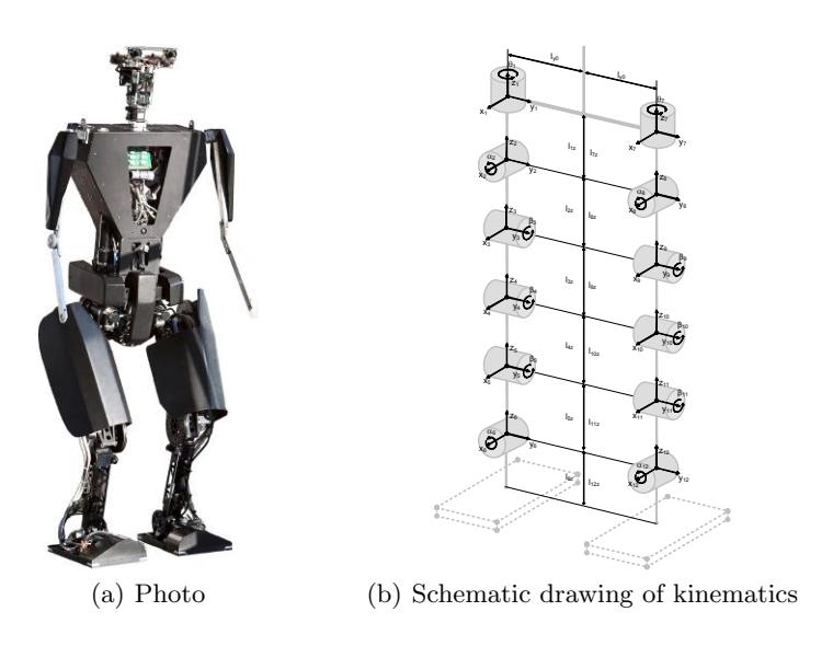
TUlip is a 134 cm tall, 30 kg heavy, anthropomorphic adult-size humanoid robot. Depicted in Fig. 1(a), TUlip has a head, a torso, two arms and two legs. The head consists of two BlackFin camera boards which enable stereo vision. The main computing unit is a 1 gHz Poseidon PC104 stack, which is placed inside the torso, together with the Mesa data acquisition boards, Elmo amplifiers and XSens 3D motion sensor which measures 3D orientation, acceleration, angular velocity and earth-magnetic field. The software on TUlip is developed in house, we do not use software from other teams. The arms of the robot comprise one degree of freedom and are placed for aesthetic reasons and for the ability to stand up after a fall. Finally, the most important parts of the humanoid robot are its legs, which both have six degrees of freedom: three revolute joints are placed in each hip, one in each knee and two in both ankles. The joints are actuated by four 90 W and eight 60 W Maxon RE30 and RE35 DC motors. On each motor a HEDS incremental encoder is placed to measure the motor axis angle. The actuators drive the joints through gearboxes with ratios between 66 and 111. Moreover, on each joint axis a Scancon incremental encoder is placed to measure the joint angle. Finally, at four points below the corners of each foot, Tekscan Flexiforce sensors are placed to measure the ground contact force. More elaborated descriptions of TUlip can be found in previous RoboCup papers [7].
Kinematically, we model TUlip as a chain of rigid bodies. As schematically depicted in Fig. 1(b), the kinematic model has six revolute joints in each leg. The dynamic equations of motion can be derived using Euler-Lagrange methods:
$$D_j(q)\ddot{q} + C_j(q,\dot{q})\dot{q} + G_j(q) = \tau, \tag{1}$$
where $q \in \mathbb{T}^{12}$ is the state vector, $D_j \in \mathbb{R}^{12 \times 12}$ is the symmetric positive definite inertia matrix, $C_j \dot{q} \in \mathbb{R}^{12}$ is the vector of Coriolis and centrifugal terms, $G_j \in \mathbb{R}^{12}$ is the gravity vector and $\tau \in \mathbb{R}^{12}$ are the joint torques. The index $j \in {R, L}$ indicates whether (1) is derived with the base coordinate frame in the right (R) or left (L) foot.
The lengths of the links of the biped are measured on the real robot. The masses, inertias and positions of the centers of mass of each link are estimated in identification experiments [5] and compared to data from the CAD drawings.
3 Walking
Gait design for humanoid robots consists of finding and controlling joint motions such that the robot can walk without falling. In this section we describe the gait design, trajectory generation and control of TUlip. Since TUlip is a heavy robot, we use statically stable gaits. A statically stable gait is a gait designed such that the robot is always in static balance, i.e. the robot always has its center of mass (CoM) within the support polygon of its feet. This type of gait is stable in the absence of environmental disturbances as long as the humanoid robot tracks the trajectories relatively slow such that any dynamic effect due to the motion of the links can be neglected.
The design of the statically stable gait consists of two parts. First, we describe how the preferred CoM and swing foot trajectories are designed in task space and secondly how these task space trajectories are mapped to joint trajectories using an inverse kinematics algorithm. Finally, we describe the controller that computes the joint torques to follow the desired gait.
3.1 Statically stable gait design
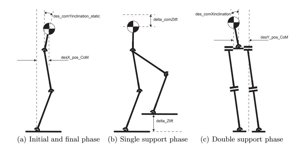
In this section we explain the design of a statically stable gait for TUlip. Each gait of TUlip consists of different phases, representing for example the initial, final, single support or double support phase. In each phase we prescribe the desired task space CoM position, torso orientation and swing foot position and orientation with respect to the stance foot. The orientations are parametrized by three angles using the roll-pitch-yaw convention.
Each phase $i \in \mathbb{N}$ has an initial posture $x_{0,i} \in \mathbb{R}^6 \times \mathbb{T}^6$ and a final posture $x_{f,i} \in \mathbb{R}^6 \times \mathbb{T}^6$ parametrized by certain variables that describe the desired task space positions and orientations. See Fig. 2 for examples of such variables. These initial and final postures are interconnected by smooth trajectories in task space described by a cosine velocity profile:
$$x_{d,i}(t) = \frac{x_{f,i} - x_{0,i}}{t_{f,i}} \left( \frac{t - \sin(\frac{2\pi}{t_{f,i}}t)}{2\pi} t_f \right) + x_{0,i}, \tag{2}$$
where $t_{f,i} \in \mathbb{R}^+$ is the duration of the phase. The total task space trajectory of the CoM and swing foot of phase i is thus given by $x_{d,i} \in \mathbb{R}^6 \times \mathbb{T}^6$ . Finally, stitching multiple phases together yield the desired task space trajectories for the entire gait:
$$x_d = \left[ x_{d,1} \dots x_{d,n} \right], \tag{3}$$
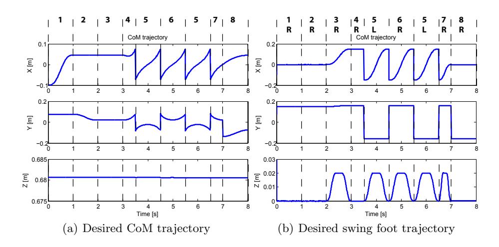
where n is the number of phases. An example of the trajectories of a statically stable gait are shown in Fig. 3. Thus, each trajectory $x_d = \begin{bmatrix} p_d^\top & \phi_d^\top \end{bmatrix}^\top$ describes six position coordinates $p_d \in \mathbb{R}^6$ of the CoM and swing foot and six orientation angles $\phi_d \in \mathbb{T}^6$ of the torso and swing foot.
3.2 Inverse kinematics
The task space trajectories defined in the previous section can be mapped to joint angles in order to control the robot in joint space. We use an inverse kinematics algorithm based on the differential kinematics:
$$\dot{x}_d = J(q_d)\dot{q}_d,\tag{4}$$
where $J \in \mathbb{R}^{12 \times 12}$ represents the geometric Jacobian of the CoM position, torso orientation and swing foot position and orientation with respect to the stance foot and $\dot{q}_d \in \mathbb{R}^{12}$ are the desired joint angular velocities, which are given by:
$$\dot{q}_d = J^{-1}(q_d)\dot{x}_d,\tag{5}$$
such that the desired joint angles $q_d \in \mathbb{T}^{12}$ are given by:
$$q_d(t) = \int_0^t \dot{q}_d(\varsigma) d\varsigma + q_d(0). \tag{6}$$
But, on a physical robot this must be implemented in discrete time and discrete integration may lead to drift. Therefore, we use an inverse kinematics algorithm proposed in [3]. Hereto, we define the error between the desired and (possibly drifted) computed task space position as:
$$e_p = p_d - p_e, (7)$$
where $p^e$ is the computed task space position of the CoM and swing foot using forward kinematics of the desired joint angles $q_d$. For the orientation we derive the desired roll-pitch-yaw rotation matrix $R^d = n^d s^d a^d$ from the desired task space orientation $\phi^d$ where $n^d$, $s^d$ and $a^d$ are simply the columns of $R^d$. Similarly, the roll-pitch-yaw rotation matrix computed by forward kinematics of the desired joint angles $q^d$ is $R^e = n^e s^e a^e$, which results in the task space orientation error:
$$e_o = \frac{1}{2}(n_e \times n_d + s_e \times s_d + a_e \times a_d). \tag{8}$$
These errors (7) and (8) are used in (5) to compensate for drift:
$$\dot{q}_d = J^{-1}(q) \begin{bmatrix} \dot{p} + K_p e_p \ L^{-1} (L^\top \omega_d + K_o e_o) \end{bmatrix}, \tag{9}$$
where
$$L = -\frac{1}{2}(S(n_d)S(n_e) + S(s_d)S(s_e) + S(a_d)S(a_e)), \tag{10}$$
with $S(\cdot)$ the skew-symmetric matrix of its vector argument. The system (9) is asymptotically stable for the positive definite matrices $K^p = \text{diag}(K_{p,1}, . . . , K_{p,6})$ and $K^o = \text{diag}(K_{o,1}, . . . , K_{o,6})$. Moreover, it can be shown that discrete time integration of (9) in (6) does not result in drift [3].
3.3 Control
The predefined joint trajectories need to be tracked on the humanoid robot such that it performs the desired gait. We describe here local feedback control on each joint to track the joint trajectories and react against disturbances. Additionally, we present a model based feedforward gravity compensation algorithm that significantly improves the tracking performance. The complete controller for system (1) is given by:
$$\tau = \tau_n + \tau_g,\tag{11}$$
where $\tau^n$ are joint controller torques and $\tau^g$ are the gravity compensation torques. We use local PD control on each joint to track the desired reference trajectories and to make the system robust against (local) disturbances:
$$\tau_n = K_P e + K_D \dot{e},\tag{12}$$
where $e = q - q^d$ are the tracking errors and $K^P = \text{diag}(K_{P,1}, . . . , K_{P,12})$ and $K^D = \text{diag}(K_{D,1}, . . . , K_{D,12})$ are the controller gains. These gains are tuned for maximal performance without destabilizing the system.
Due to the limited bandwidth of the local PD controllers, there are always feedback tracking errors in the joint angles. As a solution, we implemented a model based feedforward gravity compensation algorithm in TUlip. We use a similar heuristic approach as in [2] for computation of the gravity compensation torques for single support as well as double support. The approach is based on the ratio $\alpha$ between the distances from the CoM of the biped to its right ($\alpha = 1$) and left foot ($\alpha = 0$) respectively. The gravity compensation is now given by:
$$\tau_g = \alpha G_R(q_d) + (1 - \alpha)G_L(q_d), \tag{13}$$
where $G^R$ and $G^L$ are the gravity vectors computed in (1) with the base coordinate frame in the right, respectively the left foot. This approach automatically works in single and double support due to the parameter $\alpha$.
4 Vision, Localization and World Model
The task of image processing is to subtract features from the images produced by the cameras. Interesting features in a Robocup game are ball, goals, opponents, lines and field markers. The vision software proceeds basically as follows:
- segment by color,
- detect features in segmented image,
- apply inverse model of the lens to calculate 2D angle to each feature,
Localization consists basically of two parts. First the robot needs to localize itself on the field using vision information of the lines on the field. Secondly it determines the ball location by comparison of the diameter of the orange spot in a vision image with the known ball diameter.
The world model is responsible for maintaining information about the state of the external world. It receives sensor data from both the motion and vision modules, as well as information through the communications module. All other modules that need information on the robot state (attitude, position, viewing direction) depend on the world model. Strategy relies on the world model for performing autonomous control of the robots actions in the soccer field.
5 Strategy
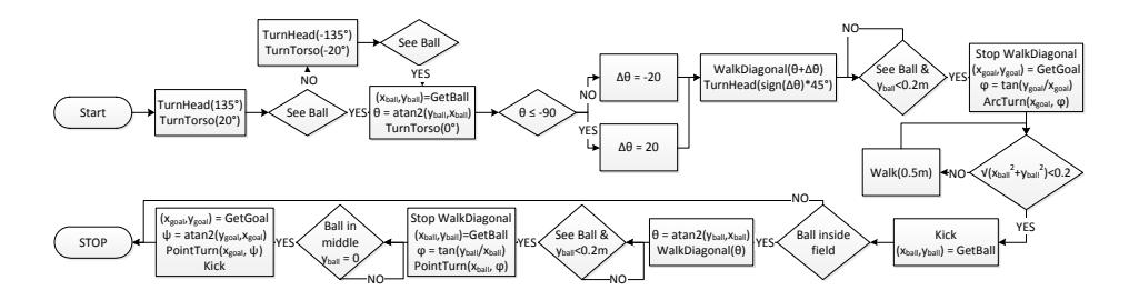
Using the gait design procedure as described in Section 3, we implemented different behaviors in TUlip such as: walking forward, walking backward, walking diagonally, side stepping, point turning and kicking. All these different behaviors and information from the world model are combined in our strategy as schematically shown in Fig. 5 for the dribble and kick challenge at the RoboCup.
In short, this strategy involves the following. First, the robot searches for the ball by turning its head and torso to the right and left. When it finds the ball it computes the distance and angle to the ball and starts moving backwards (diagonally). The robot stops when it is next to the ball where it starts turning around the ball until the ball is between the robot and the goal. The robot kicks the ball towards the goal and starts walking (diagonally) forward to the ball. Arrived at the ball, it turns again around the ball and shoots at the goal.
6 Conclusion
In this document we presented the Tech United Eindhoven adult size humanoid robot TUlip. We described its mechanical design and kinematic structure. Moreover, we explained all ingredients to achieve the dribble and kick challenge. We described the gait design and trajectory generation for statically stable walking, local feedback joint control and the feedforward gravity compensation algorithm, TUlip's vision system, self localization and world model. Finally, all these parts are used in a strategy for the dribble and kick challenge at the RoboCup 2012.
References
- D. Hobbelen, T. de Boer, and M. Wisse. System overview of bipedal robots Flame and TUlip: tailor-made for limit cycle walking. In IEEE/RSJ International Conference on Intelligent Robots and Systems (IROS), 2008, pages 2486–2491, 2008.
- S. Kajita, M. Morisawa, K. Miura, S. Nakaoka, K. Harada, K. Kaneko, F. Kanehiro, and K. Yokoi. Biped walking stabilization based on linear inverted pendulum tracking. In IEEE/RSJ International Conference on Intelligent Robots and Systems (IROS), 2010, pages 4489–4496. IEEE, 2010.
- B. Siciliano, L. Sciavicco, and L. Villani. Robotics: modelling, planning and control. Springer Verlag, 2009.
- P.W.M. van Zutven, D. Kostić, and H. Nijmeijer. On the stability of bipedal walking. LNAI series: Simulation, Modeling, and Programming for Autonomous Robots, pages 521–532, 2010.
- P.W.M. van Zutven, D. Kostić, and H. Nijmeijer. Parameter identification of robotic systems with series elastic actuators. In 8th IFAC Symposium on Nonlinear Control Systems, pages 350–355, 2010.
- P.W.M. van Zutven, D. Kostić, and H. Nijmeijer. Foot placement for planar bipeds with point feet. Proceedings of the IEEE International Conference on Robotics and Automation (ICRA), 2012.
- P.W.M. van Zutven, P. Mironchyk, C. Çilli, E. Steur, E. Ilhan, J. Caarls, R.S. Pieters, A. Filiz, P. Heijkoop, T. de Boer, A. Smorenberg, E. van Breda, G. Liqui Lung, F. Wilbers, C Plooij, G. van der Hoorn, S. Kiemel, R. Reinink, E. Dertien, G. van Oort, D. Kostić, H. Nijmeijer, M. Wisse, P.P. Jonker, R. Carloni, S. Stramigioli, and T.P.H. Warmerdam. Dutch robotics 2011 adult-size team description. 2011 Symposium papers and Team Description papers, 2011.