JiaoLong 2011 Team Description

Chuntao Leng, Qixin Cao

Research Institute of Robotics Shanghai Jiao Tong University 200240, Shanghai Dongchuan Rd No.800, P.R. China

Abstract This paper presents the improvements in hardware and fundamental control software system design of JiaoLong for RoboCup2011 competition. We propose the updated sensor data processing algorithm for vision tracking, local localization and multi-sensor data fusion algorithm for global localization. Base on the data fusion and wireless communication, we realize cooperative perception and multi-robot action coordination.

1. INTRODUCTION

The Robot World Cup Soccer Games and Conferences (RoboCup) are a series of competitions and events designed to promote the full integration of AI and robotics research. The key characteristic of middle-size league robot soccer is that the robots are completely autonomous. So it has become a standard real-world test bed for autonomous multi-robot control.

We participated in the RoboCup Competition in year 2003 for the first time, as JiaoLong Team on behalf of Shanghai JiaoTong University [1]. So we did for RoboCup 2004 and 2005. Then, Nubot associated with us to make a mixed team for RoboCup 2006. Also, we participated in RoboCup2008 in Suzhou China.

We have been putting efforts in applying a number of Behavior Learning Methods, Image Processing Methods and various cooperation algorithms, which results in the continuous enhancement of our robots. Consequently, we won all the 2:2 championship of the Middle-Size League for three times since we participated in Chinese Robot Competition (CRC) (Shanghai 2002; Beijing 2003; Guangzhou 2004; Changzhou 2005). Recently, we also got second place of 4:4 Middle-Size League in RoboCup China Open Competition (Suzhou) in 2006, and the third place of this league in RoboCup China Open Competition (Jinan) in 2007.

2. HARDWARE ARCHITECTURE

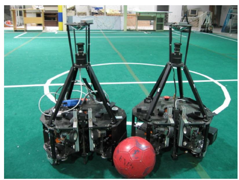
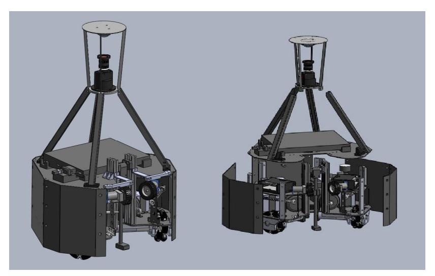
We have developed a new omni-direction robot (JL-III), which is shown in Fig1. JL-III is driven by three omni-direction wheels, which implemented with 163W hollow-cup rotor D.C. motor. It also has an omni-directional vision, one ball-handling device and a pneumatic-driving kicker, which can kick the ball with muzzle velocity of about 3m/s and over one meter height object.

For the omni-directional soccer robot, we use a laptop computer as a higher level controller for the behavior-based control. An Inter-Process Communication (IPC) mechanism is introduced to realize distributed software design, which is used to get sensor readings and to provide motor output commands and communications packet control. The TI DSP TMS320LF 2407A is adopted as a microcontroller, used for the motion control. Laptop computer and microcontroller are connected via RS-232 serial link at 19.2 Kbps. The outfield computer makes decision on the global task level as the team coordinator, while each robot executes its own sub-task assigned by team coordinator. One robot communicates with each other and the outfield PC through wireless LAN that complies with the IEEE 802.11 standard. The whole hardware system is shown in Fig.2.

The robot's maximum speed is 4 m/s and 720°/s. In the hardware device, we develop our own-made DSP control system. DSP control system process signal of motor diver, ball-handing and kicker behavior in a 1 ms circle. The laptop computer communicates with DSP in a 30 ms cycle.

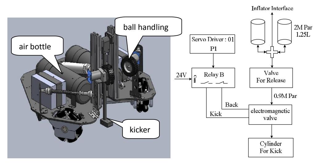
This year we developed a new kicker and ball handler system. The kicker is driven by air from two air bottle, which are 1.25L in volume and 0.9M in pressure. The mechanical and electrical architectures are shown as Fig.3. The speed of the two ball-handling motor are optimized by learning algorithm to avoid breaking rules. And the ball can be kicked as far as 7 meters.

3. IMAGE PROCESSING

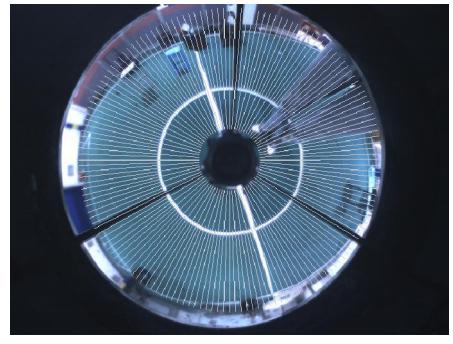
Image processing is the most time-consuming part of the program, and to advance the efficiency our image processing are based on the line scanning method. Before the image processing, we defined several line segments in the image coordinate shown as Fig.4. For each image we just scan pixels on those line segments, and detect the color transition such as the green-white-green transitions. By this way we can gather enough information and make the image processing very efficient.

Based on the line scanning information, the object recognition will be in three steps, (a) use color information to classify the color transitions into several object type, e.g., ball's transitions, white landmark line's transitions or filed transitions. (b) use some limits to filtrate useless transitions out of every transition type and (c) use Particle Filtering Algorithm to track the ball and the goal.[1]

Since in the new rules, the color goals are replaced by white nets, we changed our self-location algorithm, which was based on the colored landmarks and now the white lines. To get the location information from the white lines, we firstly use the odometer data to estimate the robot's location and digital compass data to estimate the orientation, and then use the estimated position to change the white landmark line's transitions from the image coordinate system to the world coordinate system and then match it with the real filed white lines. We model the match processing as an error minimization task and use an efficient numerical minimizer[2]. Although this algorithm is theoretically accurate, because of the vibrations of the robot, especially in the case of high velocity or due to collisions, its accuracy is badly affected. So we use a Kalman filter to track and smooth the position and calculate several explicit alternative positions to alter the main position if it's necessary. Experiments show that the position error of robot's self-localization can be less than 50cm.

4. MOTION CONTROL SYSTEM

4.1 Motion Characteristics Analysis [4]

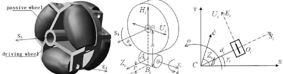
To design a robot with good performance, it is necessary to build the kinematic model for analyzing the velocity characteristics of the omni-directional mobile robot. According to the velocity relationship of the driving roller and the passive roller as shown in Fig.4, the velocity of the driving roller centre can be determined by:

$$\dot{o}_i = -R\dot{\theta}_i U_i - r\dot{\phi}_i Z_i$$ (1)

Meanwhile the velocity also can be denoted by the velocity of robot centre ( ) and angular velocity ω , and the equation is:

$$\dot{o}_i = \dot{c} + \omega \xi d_i \text{ where } \xi \equiv \begin{bmatrix} 0 & -1 \ 1 & 0 \end{bmatrix}$$ (2)

Due to the passive rollers not being driven by a motor, the angular velocity of the passive roller is irrelevant to our study, and can be eliminated during kinematic analysis.

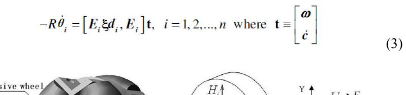
Dot-multiplied by the axle vector on both sides of equation (1) and (2), we can derive equation (3) as a general kinematic equation for the OMR:

4.2 Control system

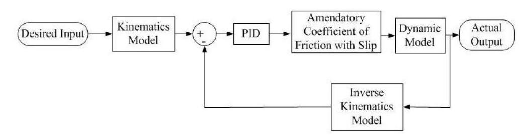
By using the derived dynamic model, the PID based control system for the OMR has been developed, as shown in Fig.6. This system modulates the velocity of each wheel at any moment with interpolation to achieve the given target position and velocity of the robot.

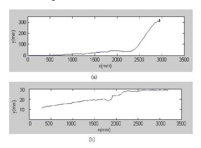
In order to check the property of the robot, a pure X translational motion was commanded in experiment with the linear speed of 1500mm/s. Figure 7 shows the corresponding x and y position of the robot. Figure 7 (a) is the result without considering the effect of slipping and (b) shows the result based on the improved friction model given above. Comparing with these two experimental data, when one unexpected impact encountered in x=2350mm (Fig. 7 (a)) and in x=1850mm (Fig. 7 (b)) respectively, the result with the new, improved friction model showed that the slipping for Y translational motions was not as severe as the former, which demonstrates the feasibility of our analysis.

5. TRAJECTORY PLANNING

In order to accurately and effectively avoid the obstacles and reach the goal, we propose a more suitable motion planning for OMR. A revolving factor is introduced into the APF for the evolutional APF. The revolving factor in addition to considering the anisotropy of OMR, the impact of the dynamic information of obstacles and goal are also important. The consideration of relative movement among robot, obstacles and goal will be better to improve the efficiency [4] .

5.1 Effect of obstacles

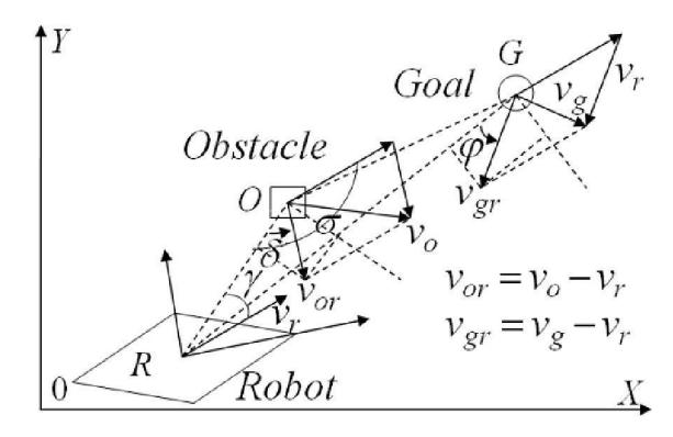
As shown in fig.8, suppose that the velocity of robot is ^r v , the velocity of obstacle is ^o v , and the velocity of goal is ^g v . The relative velocity between robot and obstacle is or v , and the relative velocity between robot and goal is gr v . is the angle between ^r v and OR. is the angle between or v and OR. is a supplementary angle of . is the angle between gr v and RG. All these angles take counter-clockwise as positive direction. In the use of revolving factor to coordinate the APF force and to achieve much more high-speed motion planning, consideration of dynamic information of obstacles is very important. When is less than , the obstacle is moving to the direction of robot movement, i.e. the behavior for avoiding collision is necessary; And when is greater than , the obstacle is moving away from robot, i.e. the behavior for avoiding collision is not necessary.

When the distance between the robot and the obstacle is less than some threshold, it should avoid them deceasing, and also the appearance of the obstacle in the direction of robot movement should be avoided. Obviously when the distance between the robot and the obstacle is greater than some threshold, there is no need to avoid collision. To achieve the above objective, we can increase the velocity in the vertical direction of OR, which means to increase the coordinating angle. Without the threat of obstacles, the velocity in the vertical direction of OR should be defined depending on the improving the speed of motion planning. At the relative velocity or v , the time needed when robot runs into obstacle and the time needed when obstacle moves to the direction of robot movement, are noted as an impact factor to define the coordinating angle. And it can be modeled as (4). Where ¹ n and 2 n are the coordinating parameters.

$$\theta_{rel-O} = n_1 D_{or} / (v_{or} \cos \delta) + n_2 D_{or} \gamma / (v_{or} \sin \delta)$$ (4)

5.2 Effect of the goal

In order to reach the goal with much more high-efficiency, i.e. the motion planning is not a simple tracking but an effective interception, the relative movement tendency between robot and goal should be considered. It is obvious that the coordinating angle depends on the velocity component of gr v in the vertical of RG, i.e. the faster the velocity component is, the bigger the coordinating angle will be. And with the coordinating angle resulted from the movement of goal, the robot can predict the future position of goal and directly go to there. When the velocity component of gr v in the direction of RG is small, the time spent for the distance of RG will be short, accordingly the coordinating angle should be small. According to the above analysis, to capture the goal with high-efficiency, the coordinating angle resulted from the relative velocity between robot and goal can be modeled as (5). Where 3 n and 4 n are the coordinating parameters.

$$\theta_{rel-G} = n_3 v_{gr} \sin \varphi + n_4 D_{rg} / (v_{gr} \cos \varphi)$$ (5)

Therefore, for a short trajectory, a high-speed, stable-acceleration, collision avoidance motion planning with high efficiency, it can be achieved by adjusting the coordinating parameters, i.e. by adjusting the proportion of impact factor, the perfect trajectory can be achieved. With above analysis, finally the total APF force ( $\boldsymbol{A}$ ) is shown in (6).

$$\mathbf{A} = (\mathbf{F}{att} + \mathbf{F}{ren}) \cdot e^{j(\theta_v + \theta_a + \theta_{rel-O} + \theta_{rel-G})}$$ (6)

5.3 Results

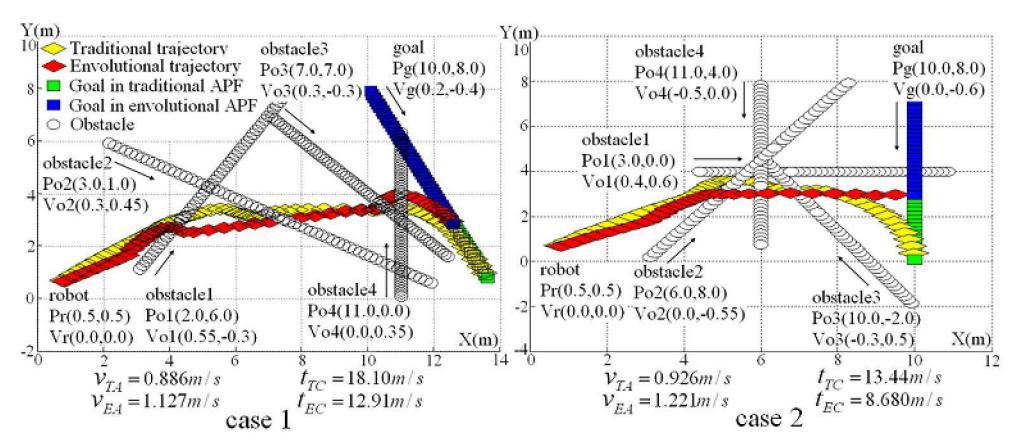
In respect of APF, there are different approaches to get the velocity to control the motion of robot. In our research to exert the advantage of OMR, the total APF force only determines the direction of robot motion. Due to the security reasons, the robot runs at maximum velocity while far away from the obstacles, and it decelerates while the distance from obstacles is smaller than some threshold, with the velocity in proportion to the relative distance. And when the robot does not run at maximum velocity, the revolving factor will not function. The simulation results are shown in Fig.9.

6. BEHAVIOR CONTROL

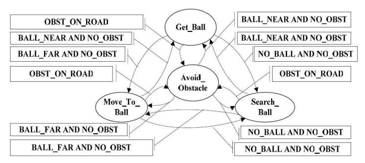
Firstly, each robot's behavior control is designed according to FSA and Motor Schema theory [6, 7]. Every robot has the following basic behaviors: Dribble_Ball, Move_To_Goal, Search_Goal, Shoot_Ball and Avoid_Obstacle. Multiple behaviors fusion is realized by summation of activated behavior vectors, as shown in Fig.10.

Secondly, we couple the behavior systems of the robots by a team communication mechanism. Via WLAN, the team players submit their model parameters and states to the team coordinator periodically; the outfield computer fuses out global model. Through one dynamic role assignment strategy, the outfield computer updates the new role assignment and team state of each robot. That is, the role is not fixed but varies according to the ball position. Through these two strategies, we can realize robots behavioral control and cooperation.

7. CONCLUSION

In this paper we presented the hardware and control software design of JiaoLong for RoboCup2011 competition. The image processing method are mentioned here for robot's global localization in MSL. Especially, we introduce the and motion control and trajectory planning method for robot's control and try to apply omni-directional wheel to make the robot move smoothly. An FSM-based behavior selection method is used to solve multi-behavior coordination problem. Base on the data fusion and wireless communication, we realize cooperative perception and multi-robot action coordination.

References

1. Weidong Chen, Qixin Cao, and et al: "JiaoLong2003 Team Description" RoboCup Soccer Middle-Size League, RoboCup2003, Padua, Italy, 5-9 July 2003.
2. A. Merke, S. Welker and M. Riedmiller: Line base robot localisation under natural light conditions, In ECAI Workshop on Agents in Dynamic and Real-Time Environments, 2004
3. Martin Lauer, Sascha Lange and Martin Riedmiller: Calculating the perfect match: An efficient and accurate approach for robot self-localisation. In A. Bredenfeld, A. Jacoff, I. Noda and Y. Takahashi, editors, RoboCup 2005: Robot Soccer World Cup IX, LNCS. Springer, 2005
4. Chuntao Leng, Qixin Cao, Charles Lo , A motion control method for omni-directional mobile robots based on anisotropy , Industrial Robot: An International Journal,37/1 (2010), PP.23–35
5. Cao Qixin, Leng Chuntao, Huang Yanwen. An evolutional artificial potential field algorithm based on the anisotropy of omnidirectional mobile robot, ICMIT2007, The 2007 International Conference on Mechatronics and Information Technology, December 5-6, 2007, Gifu, Japan
6. J. Connell: "SSS: A Hybrid Architecture Applied To Robot Navigation" IEEE Int. Conf. Robotics and Automation, 1992.
7. R. C. Arkin: "Motor Schema-Based Mobile Robot Navigation" International Journal of Robotics research, Vol. 8, pp. 92-112, 1987.