The magmaOffenburg 2014 RoboCup 3D Simulation Team

Klaus Dorer, Stefan Glaser

Hochschule Offenburg, Elektrotechnik-Informationstechnik, Germany

Abstract This paper describes the magmaOffenburg 3D simulation team trying to qualify for RoboCup 2014. While last year's TDP focused on how we statistically evaluate new features, this year we focus on our Trunk controlled Motion Framework used for walking and kicking.

Introduction

A major step forward for the magmaOffenburg team has been the introduction of the Trunk controlled Motion Framework (TcMF). It is a separate component that allows to specify any motion for the legs that needs to be stabilized. It separates motion definition from any adjustments necessary in case of deviations from the desired trunk orientation. This makes motion definition easier, yet produces significantly better results in the 3D soccer simulation environment.

Section 2 explains the TcMF in detail. In section 3 we present two applications of the framework, walking and stoping on one leg. Section 4 gives some results of applying the TcMF.

Trunk Controlled Motion Framework

The idea behind the Trunk controlled Motion Framework (TcMF) follows a simple thought: A balanced motion should always support the center of mass. In order to achieve this, motions should be defined with respect to a reference frame with the center of mass as its origin. Furthermore supporting the center of mass usually means acting against gravity, regardless of the actual tilt of the robot. The orientation of the reference frame should therefore always point upright, but still facing the horizontal view direction of the robot. We call this reference frame $Motion\ Frame\ \mathcal{M}$ .

So far we simply switched the reference frame in which we define the motions from the local trunk frame $\mathcal{T}$ to the virtual Motion Frame. In order to use an inverse kinematics solver, we now need to transform the motion trajectories back into the trunk frame, using the following equation:

$$\mathbf{T}{l}^{\mathcal{T}} = \mathbf{T}{\mathcal{M}}^{\mathcal{T}} \ \mathbf{T}_{l}^{\mathcal{M}} \tag{1}$$

where $\mathbf{T}_l^{\mathcal{M}}$ and $\mathbf{T}l^{\mathcal{T}}$ expresses the pose of limb l with respect to frame $\mathcal{M}$ respectively $\mathcal{T}$ . The transformation $\mathbf{T}{\mathcal{M}}^{\mathcal{T}}$ from the Motion Frame to the trunk follows directly from the definition:

$$\mathbf{T}{\mathcal{M}}^{\mathcal{T}} = \begin{bmatrix} \mathbf{R}{\mathcal{M}}^{\mathcal{T}} \ \mathbf{t}_{CoM}^{\mathcal{T}} \ \mathbf{0} & 1 \end{bmatrix}$$ (2)

where $\mathbf{R}{\mathcal{M}}^{\mathcal{T}}$ describes the current tilt of the trunk and $\mathbf{t}{CoM}^{\mathcal{T}}$ the position of the CoM with respect to the trunk frame. By using a static CoM position together with the identity rotation to construct $\mathbf{T}_{\mathcal{M}}^{\mathcal{T}}$ , we end up with the same local motion as we had before. However, by using the current estimation for tilt and CoM to transform the motion trajectories, we get a motion which is automatically adjusted to the current CoM and tilt of the robot.

The current tilt is obtained from the orientation $\mathbf{R}_{\mathcal{T}}^{\mathcal{W}}$ of the trunk with respect to the world frame $\mathcal{W}$ by removing the horizontal rotation part of the orientation:

$$\mathbf{R}{\mathcal{T}}^{\mathcal{M}} = \mathbf{R}{\mathcal{W}}^{\mathcal{M}} \ \mathbf{R}_{\mathcal{T}}^{\mathcal{W}} \tag{3}$$

where $\mathbf{R}_{\mathcal{W}}^{\mathcal{M}}$ by definition is the rotation around the z-axis about the horizontal view angle of the robot. In our case, the current tilt of the robot corresponds to the orientation of the trunk with respect to the Motion Frame. In order to plug formula 3 into 2, we need to invert formula 3:

$$\mathbf{R}{\mathcal{M}}^{\mathcal{T}} = (\mathbf{R}{\mathcal{T}}^{\mathcal{M}})^{-1} = (\mathbf{R}{\mathcal{W}}^{\mathcal{M}} \ \mathbf{R}{\mathcal{T}}^{\mathcal{W}})^{-1} \tag{4}$$

So far motions are closed-loop in the sense that trajectories of legs are adjusted to any tilt of the trunk and movement of the CoM. However, they are not counteracting any tilt of the robot. If the orientation estimation of the robot would be perfect, this tilt adjustment would basically try to preserve the current tilt of the trunk. In order to continuously push the current z-axis of the trunk upright (towards the global z-axis), we can manipulate $\mathbf{R}_{\mathcal{M}}^{\mathcal{T}}$ by applying an additional rotation, interpolating from the actual z-axis of the trunk to the global z-axis. The resulting adapted trunk frame is called $\mathcal{T}$ .

$$\mathbf{R}{\mathcal{M}}^{\mathcal{T}'} = \mathbf{R}{\mathcal{T}}^{\mathcal{T}'} \ \mathbf{R}_{\mathcal{M}}^{\mathcal{T}} \tag{5}$$

If we now use this manipulated tilt estimation $\mathbf{R}{\mathcal{M}}^{\mathcal{T}'}$ in formula 2 to construct $\mathbf{T}{\mathcal{M}}^{\mathcal{T}'}$ and plug $\mathbf{T}{\mathcal{M}}^{\mathcal{T}'}$ into formula 1 to transform the motion trajectories into $\mathcal{T}'$ , we get a motion that is not only adjusted to the current CoM and tilt of the robot, but also continuously trying to push the trunk upright. The amount by how much we interpolate between the current and upright situation specifies the weighting between the two adjustments. Zero percent interpolation ( $\mathcal{T}' = \mathcal{T} \to \mathbf{R}{\mathcal{T}}^{\mathcal{T}'} = \mathbf{R}{\mathcal{T}}^{\mathcal{T}} = \mathbf{I}$ ) results solely in the first tilt adjustment. Whereas 100 percent interpolation ( $\mathcal{T}' = \mathcal{M} \to \mathbf{R}{\mathcal{T}}^{\mathcal{T}'} = \mathbf{R}_{\mathcal{T}}^{\mathcal{M}}$ ) would simply cancel out the first tilt adjustment, with the consequence that the motion is still related to the current CoM, but without any further adjustment to the current tilt of the trunk. Any interpolation in between describes a trade off between adapting to the current tilt and pushing the trunk upright.

The interpolation rotation $\mathbf{R}{\mathcal{T}}^{\mathcal{T}'}$ can be constructed in different ways. A simple method to construct $\mathbf{R}{\mathcal{T}}^{\mathcal{T}'}$ is using a quaternion slerp between $\mathcal{T}$ and $\mathcal{M}$ . However, a quaternion slerp entails an implicit weighting between the Sagittal and Coronal adjustment, which restricts the flexibility of the controller. We therefore use the Euler/Cardan angles convention to describe the difference from $\mathcal{T}$ to $\mathcal{M}$ , which implicitly requires the separation of $\mathbf{R}^{\mathcal{M}}{\mathcal{T}}$ into three elemental rotations. Since we only consider the tilt of the trunk without the horizontal direction, $\mathbf{R}^{\mathcal{M}}{\mathcal{T}}$ can be composed by only two elemental rotations, one around the x-axis (Sagittal axis) and one around the y-axis (Coronal axis), which can be interpolated separately. The interpolation itself is realized by a simple proportional controller.

Until now, the above described framework tries to maintain an upright direction of the trunk. While this may be sufficient to support for example a walking motion, it lacks flexibility with respect to general motions, which may intend to maintain a specific tilt, different from upright. However, extending the above framework to maintain an arbitrary tilt is straight forward. The second adjustment, responsible for maintaining an upright state, is constructed by an interpolation between the current state $\mathcal{T}$ and the upright situation $\mathcal{M}$ . More precisely by an interpolated rotation between the current z-axis of the trunk and the global z-axis. By switching the interpolation target from the global z-axis to an arbitrary unit vector, we can guide the second adjustment towards maintaining an arbitrary tilt. We call this unit vector describing the intended tilt of the trunk (intended) leaning vector. With the requirement to specify an intended leaning vector to the TcMF, each motion automatically describes its own adjustment target. More details can be found in [1].

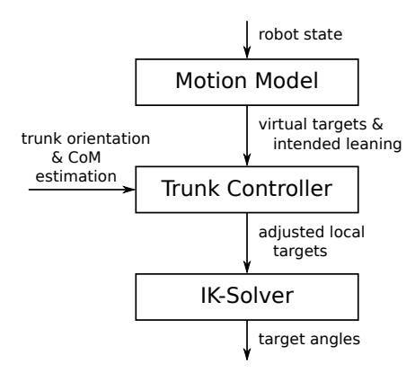
A motion using the TcMF typically consists of three components (Figure 1):

Fig. 1. Component diagram of a motion using the TcMF.

Applications

In this section we show two applications of the TcMF, (omnidirectional) walking and stopping balanced on one leg (for kicking).

Walking

The walk motion consists of a simple trajectory of a linear movement for the support leg and a sinoidal movement for the free leg. The walk is specified as an 18 cycle (50 Hz) motion so a complete step cycle takes 0.36 s. The trajectory has been optimized to the maximum motor speed of the simulated Nao of 7.03 degrees per 20 ms. Only in 3 of the 18 cycles the inverse kinematics is not limited by the maximum speed.

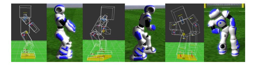
Independent from this trajectory, a torso leaning can be specified. Figure 2 shows two examples of static leaning definitions. Images three and four show a 30 degree forward leaning while walking forward at 0.8 m/s. Images five and six show a 20 degree sideward leaning while walking forward at 0.5 m/s. The CoM is shown as an olive circle in the wire frames. Dynamic leaning definitions are possible. A more natural example would be to lean forward dependent on the forward acceleration of the robot.

Fig. 2. Walk as an application of the TcMF. Image one and two: Nao upright. Image three and four: walking with 30 degrees forward leaning. Image five and six: walking with 20 degrees sideward leaning.

One Leg Stopping

A considerable amount of time can be saved for kicking, if the robot does not have to stop on both legs before kicking. It also makes it possible to place the support foot at the side of the ball. This section describes how TcMF is used to stop on one leg and keeping balance for kicking.

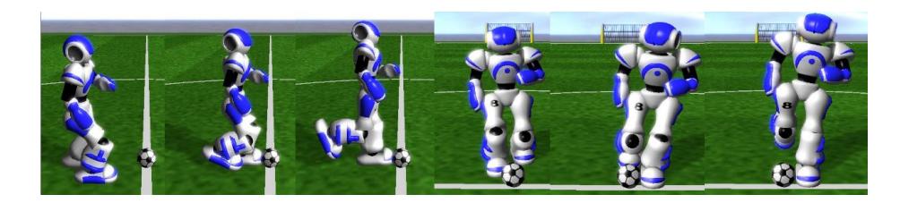
One leg stopping is divided into three motions: a final step motion, a get on leg motion and a balance on leg motion. The final step motion is defined by the ball relative position of the support foot, the desired global kick direction and which of the two legs should be support foot. The motion itself makes sure to turn appropriately. Since the Nao robot is not able to do inward turns, any remaining turn angle to the right, if the final support foot is the right foot, have to be done with the second last step. The get on leg motion performs the final step and specifies an appropriate trunk leaning. It also makes sure that the free foot is started to be moved towards a kicking position. Finally, it also performs any remaining turn to the desired kick direction. The balance on leg motion finally stabilizes the robot standing already on one leg, adjusts the height of the hip to proper kick height and defines the final trunk leaning required for the kick. The kick itself is currently performed in joint space outside the TcMF. The end of each motion is shown in Figure 3 for a straight kick.

Fig. 3. Stop on one leg as an application of the TcMF. First image: end of final step motion. Second image: end of get on leg motion. Third image: end of balance on leg motion. Fourth to Sixth image: same from front.

Results

Experiments in this section have been conducted with the RoboCup 3D soccer simulation server version 0.6.6 [5] on a simulated Nao robot.

Walking

To demonstrate the effectiveness of TcMF a first experiment let the robot walk forward for four seconds with a speed of 0.5 m/s. The first two seconds the desired torso leaning was set to 30 degrees forward leaning. The last two seconds the desired torso leaning was upright again to see how effective the trunk controller can adjust to the new leaning.

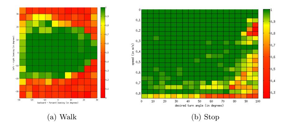
Figure 4 shows the range of torso rotations in which the robot is still able to walk. The setup is like above, 2 seconds walking with a leaning followed by two seconds walking upright. The leaning was varied from 30 degrees backward leaning to 30 degrees forward leaning and for each of these values also from 30 degrees left to 30 degrees right leaning. Each point is the average of 40 runs counting the average probability not to fall down.

The robot is able to walk with 30 degrees forward and 25 degrees backward leaning, if there is no sideward leaning. It is also able to walk with 20 degrees side leaning in both sides if there is no forward-backward leaning. Even a 15 degrees forward and sideward leaning can be sustained while walking and corrected upright when desired after two seconds.

One Leg Stopping

To evaluate stopping on one leg, the robot walked straight for 1.4 seconds and then stopped on the left leg. We varied the speed at which the robot was walking from 0 to 0.85 m/s and the desired horizontal turn angle from 0 to 100 degrees. Each result is an average of 40 trials. Figure 4 right shows the reliability of the one leg stopping motions. Even with 0.8 m/s the robot is able to stop on one leg reliably for a range of turn angles. For a considerable speed of 0.6 m/s an effective turn of 50 degrees is reliably achievable.

Fig. 4. Probability of not falling down when walking with different leanings (a) and stopping at different speeds and with different turn angles (b).

References

Glaser S and Dorer K (2013) Trunk Controlled Motion Framework. In Proceedings of the 8th Workshop on Humanoid Soccer Robots, IEEE-RAS International Conference on Humanoid Robots, Atlanta, 2013.
Hochberg U, Dietsche A and Dorer K (2013) Evaporative Cooling of Actuators for Humanoid Robots. In Proceedings of the 8th Workshop on Humanoid Soccer Robots, IEEE-RAS International Conference on Humanoid Robots, Atlanta, 2013
Schindler, I.: Laufen auf zwei Beinen in der simulierten RoboCup 3D-Umgebung. Bachelor thesis, Hochschule Offenburg, Germany (2009)
Dorer, K.: Modeling Human Decision Making using Extended Behavior Networks. J Baltes et al. (Eds.): RoboCup 2009, LNAI 5949, pp. 81–91. Springer (2010)
O. Obst and M. Rollmann, SPARK A Generic Simulator for Physical Multiagent Simulations Computer Systems Science and Engineering, 20(5), September 2005
Dorer, K.: Extended Behavior Networks for Behavior Selection in Dynamic and Continuous Domains. In: U. Visser, et al. (Eds.) Proceedings of the ECAI workshop Agents in dynamic domains, Valencia, Spain (2004)
Dorer, K.: Behavior Networks for Continuous Domains using Situation–Dependent Motivations. Proceedings of the Sixteenth International Conference of Artificial Intelligence (1999) 1233–1238